Calcium Imaging#
Working with calcium data.
As example dataset, we will be working with a recording of a freely-moving mouse imaged with a Miniscope (1-photon imaging). The area recorded for this experiment is the postsubiculum - a region that is known to contain head-direction cells, or cells that fire when the animal’s head is pointing in a specific direction.
The NWB file for the example is hosted on OSF. We show below how to stream it.
Downloading the data#
First things first: let’s find our file.
path = "A0670-221213.nwb"
if path not in os.listdir("."):
  r = requests.get(f"https://osf.io/sbnaw/download", stream=True)
  block_size = 1024*1024
  with open(path, 'wb') as f:
    for data in r.iter_content(block_size):
      f.write(data)
Parsing the data#
Now that we have the file, let’s load the data:
data = nap.load_file(path, lazy_loading=False)
data
A0670-221213
┍━━━━━━━━━━━━━━━━━━━━━━━┯━━━━━━━━━━━━━┑
│ Keys                  │ Type        │
┝━━━━━━━━━━━━━━━━━━━━━━━┿━━━━━━━━━━━━━┥
│ position_time_support │ IntervalSet │
│ RoiResponseSeries     │ TsdFrame    │
│ z                     │ Tsd         │
│ y                     │ Tsd         │
│ x                     │ Tsd         │
│ rz                    │ Tsd         │
│ ry                    │ Tsd         │
│ rx                    │ Tsd         │
┕━━━━━━━━━━━━━━━━━━━━━━━┷━━━━━━━━━━━━━┙
Let’s save the RoiResponseSeries as a variable called ‘transients’ and print it:
transients = data['RoiResponseSeries']
transients
Time (s)          0        1         2         3         4  ...
----------  -------  -------  --------  --------  --------  -----
3.1187      0.27546  0.79973  0.16383   0.20118   0.029255  ...
3.15225     0.26665  0.86751  0.15879   0.23682   0.027189  ...
3.18585     0.25796  0.89419  0.15352   0.25074   0.036514  ...
3.2194      0.24943  0.89513  0.14812   0.25215   0.056273  ...
3.253       0.24111  0.88023  0.14898   0.24651   0.070954  ...
3.28655     0.233    0.85584  0.14858   0.23706   0.081469  ...
3.32015     0.22513  1.0996   0.14715   0.22572   0.088588  ...
...                                                         ...
1203.38945  0.20815  0.17535  0.12126   0.094461  0.87427   ...
1203.42305  0.20247  0.17243  0.11807   0.089918  1.2578    ...
1203.4566   0.19654  0.17056  0.11461   0.085079  1.62      ...
1203.4902   0.19052  0.16645  0.11096   0.080197  1.8811    ...
1203.52375  0.18449  0.16105  0.10717   0.075416  2.0599    ...
1203.55735  0.17851  0.15494  0.10331   0.070814  2.2176    ...
1203.5909   0.17264  0.14851  0.099416  0.066429  2.311     ...
dtype: float64, shape: (35757, 65)
Plotting the activity of one neuron#
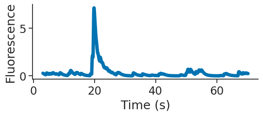
Our transients are saved as a (35757, 65) TsdFrame. Looking at the printed object, you can see that we have 35757 data points for each of our 65 regions of interest (ROIs). We want to see which of these are head-direction cells, so we need to plot a tuning curve of fluorescence vs head-direction of the animal.
plt.figure(figsize=(6, 2))
plt.plot(transients[0:2000,0], linewidth=5)
plt.xlabel("Time (s)")
plt.ylabel("Fluorescence")
plt.show()
Here, we extract the head-direction as a variable called angle.
angle = data['ry']
angle
Time (s)
----------  -------
3.0994      2.58326
3.10775     2.5864
3.11605     2.5905
3.1244      2.59191
3.13275     2.59263
3.14105     2.59306
3.1494      2.59404
...
1206.1728   3.70308
1206.18115  3.6908
1206.18945  3.69804
1206.1978   3.6728
1206.20615  3.65452
1206.21445  3.61199
1206.2228   3.5495
dtype: float64, shape: (144382,)
As you can see, we have a longer recording for our tracking of the animal’s head than we do for our calcium imaging - something to keep in mind.
transients.time_support
  index    start      end
      0   3.1187  1203.59
shape: (1, 2), time unit: sec.
Calcium tuning curves#
Here, we compute the tuning curves of all the ROIs.
tuning_curves = nap.compute_tuning_curves(transients, angle, bins=120)
tuning_curves
<xarray.DataArray (unit: 65, 0: 120)> Size: 62kB
array([[0.39569942, 0.27969522, 0.39860297, ..., 0.26886614, 0.28176322,
        0.29267547],
       [0.05584286, 0.05242977, 0.04442249, ..., 0.06026938, 0.06446022,
        0.04855164],
       [0.15030357, 0.15392468, 0.20111337, ..., 0.12047493, 0.13192547,
        0.11677392],
       ...,
       [0.08680351, 0.09815416, 0.08971635, ..., 0.12115679, 0.09941108,
        0.09034233],
       [0.09039302, 0.11255827, 0.0925766 , ..., 0.09920906, 0.09860094,
        0.08435247],
       [0.09093062, 0.10119966, 0.12785623, ..., 0.08399268, 0.08817498,
        0.09970528]], shape=(65, 120))
Coordinates:
  * unit     (unit) int64 520B 0 1 2 3 4 5 6 7 8 ... 56 57 58 59 60 61 62 63 64
  * 0        (0) float64 960B 0.0262 0.07856 0.1309 0.1833 ... 6.152 6.205 6.257
Attributes: (3)This yields an xarray.DataFrame, which we can beautify by setting feature names and units:
def set_metadata(tuning_curves):
_tuning_curves=tuning_curves.rename({"0": "Angle", "unit": "ROI"})
_tuning_curves.name="Fluorescence"
_tuning_curves.attrs["units"]="a.u."
_tuning_curves.coords["Angle"].attrs["units"]="rad"
return _tuning_curves
annotated_tuning_curves = set_metadata(tuning_curves)
annotated_tuning_curves
<xarray.DataArray 'Fluorescence' (ROI: 65, Angle: 120)> Size: 62kB
array([[0.39569942, 0.27969522, 0.39860297, ..., 0.26886614, 0.28176322,
        0.29267547],
       [0.05584286, 0.05242977, 0.04442249, ..., 0.06026938, 0.06446022,
        0.04855164],
       [0.15030357, 0.15392468, 0.20111337, ..., 0.12047493, 0.13192547,
        0.11677392],
       ...,
       [0.08680351, 0.09815416, 0.08971635, ..., 0.12115679, 0.09941108,
        0.09034233],
       [0.09039302, 0.11255827, 0.0925766 , ..., 0.09920906, 0.09860094,
        0.08435247],
       [0.09093062, 0.10119966, 0.12785623, ..., 0.08399268, 0.08817498,
        0.09970528]], shape=(65, 120))
Coordinates:
* ROI (ROI) int64 520B 0 1 2 3 4 5 6 7 8 9 ... 56 57 58 59 60 61 62 63 64
* Angle (Angle) float64 960B 0.0262 0.07856 0.1309 ... 6.152 6.205 6.257
Attributes: (4)Having set some metadata, we can easily plot one ROI:
annotated_tuning_curves[4].plot()
plt.show()
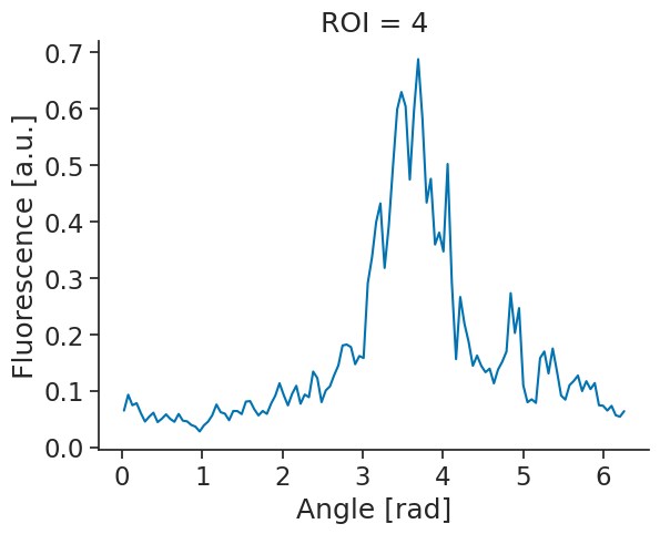
It looks like this could be a head-direction cell. One important property of head-directions cells however, is that their firing with respect to head-direction is stable. To check for their stability, we can split our recording in two and compute a tuning curve for each half of the recording.
We start by finding the midpoint of the recording, using the function get_intervals_center. Using this, then create one new IntervalSet with two rows, one for each half of the recording.
center = transients.time_support.get_intervals_center()

halves = nap.IntervalSet(
    start = [transients.time_support.start[0], center.t[0]],
    end = [center.t[0], transients.time_support.end[0]]
)
/tmp/ipykernel_2309/1625859845.py:3: UserWarning: Some starts and ends are equal. Removing 1 microsecond!
  halves = nap.IntervalSet(
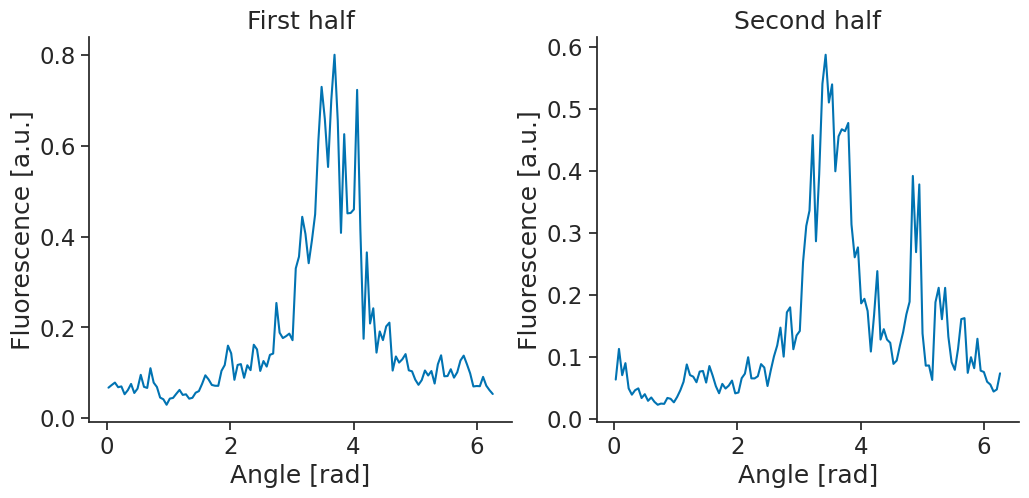
Now, we can compute the tuning curves for each half of the recording and plot the tuning curves again.
tuning_curves_half1 = nap.compute_tuning_curves(transients, angle, bins = 120, epochs = halves.loc[[0]])
tuning_curves_half2 = nap.compute_tuning_curves(transients, angle, bins = 120, epochs = halves.loc[[1]])

fig, (ax1, ax2) = plt.subplots(1, 2, figsize=(12, 5))
set_metadata(tuning_curves_half1[4]).plot(ax=ax1)
ax1.set_title("First half")
set_metadata(tuning_curves_half2[4]).plot(ax=ax2)
ax2.set_title("Second half")
plt.show()
Calcium decoding#
Given some tuning curves, we can also try to decode head direction from the population activity.
For calcium imaging data, Pynapple has decode_template, which implements a template matching algorithm.
epochs = nap.IntervalSet([50, 150])
transients = transients.bin_average(0.1)
decoded, dist = nap.decode_template(
    tuning_curves=tuning_curves,
    data=transients,
    epochs=epochs,
    bin_size=0.1,
    metric="correlation",
)
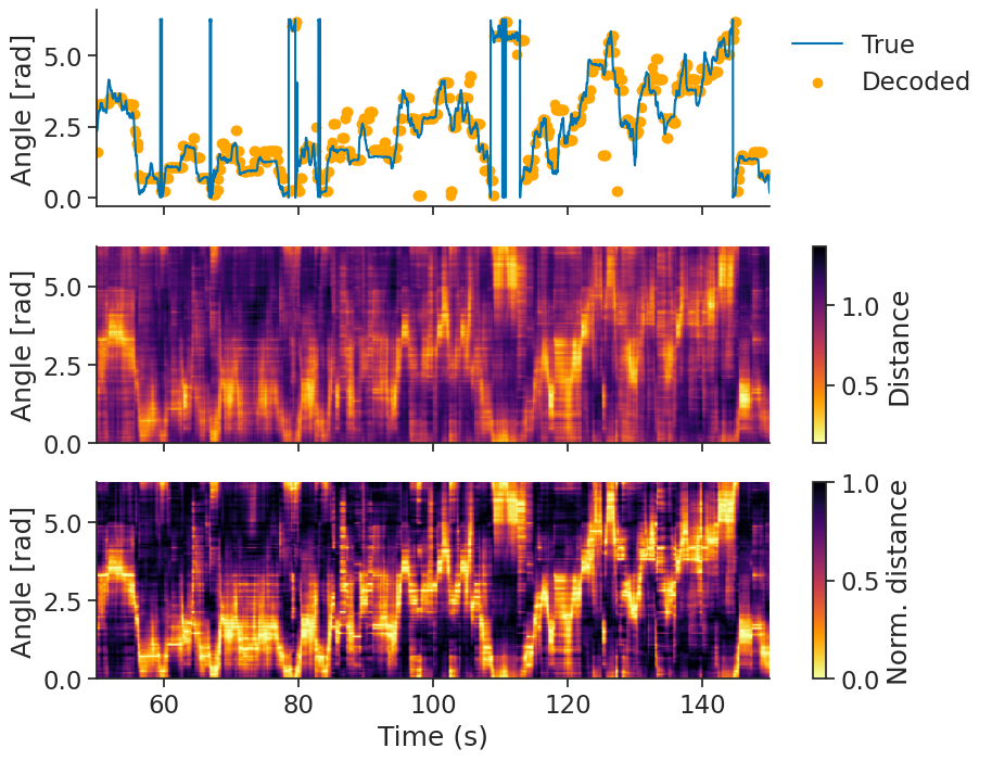
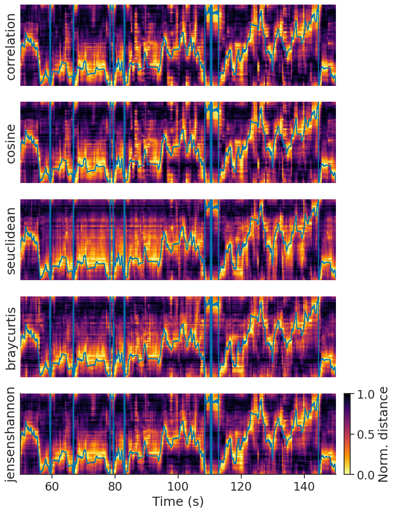
The distance metric you choose can influence how well we decode.
Internally, decode_template uses scipy.spatial.distance.cdist to compute the distance matrix;
you can take a look at its documentation
to see which metrics are supported. Here are a couple examples:
We recommend trying a bunch to see which one works best for you. In the case of head direction, we can quantify how well we decode using the absolute angular error. To get a fair estimate of error, we will compute the tuning curves on the first half of the data and compute the error for predictions of the second half.
def absolute_angular_error(x, y):
    return np.abs(np.angle(np.exp(1j * (x - y))))

# Compute errors
errors = {}
for metric in metrics:
    decoded, dist = nap.decode_template(
        tuning_curves=tuning_curves_half1,
        data=transients,
        bin_size=0.1,
        metric=metric,
        epochs=halves.loc[[1]],
    )
    errors[metric] = absolute_angular_error(
        angle.interpolate(decoded).values, decoded.values
    )
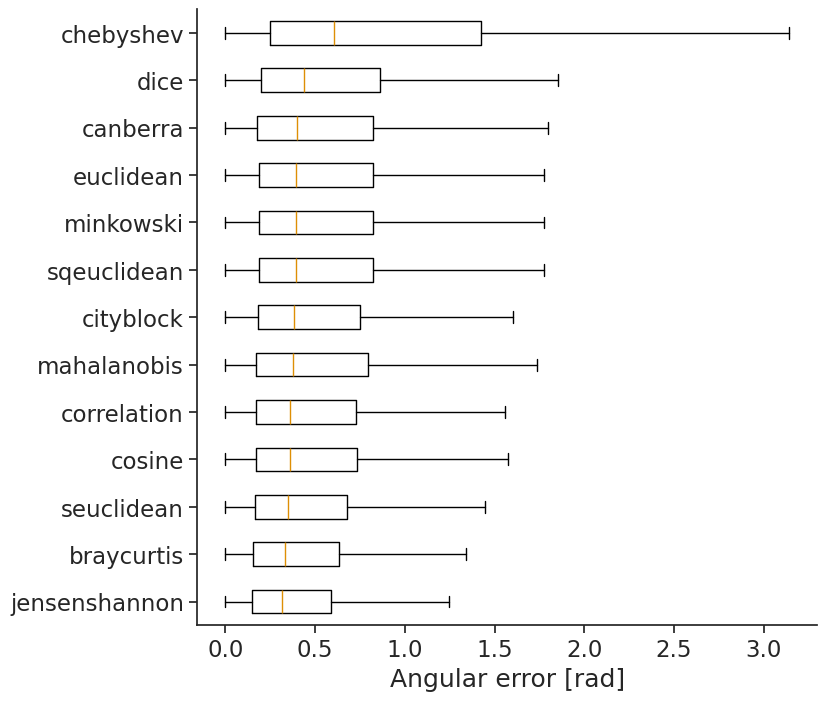
In this case, jensenshannon yields the lowest angular error.
Authors
Sofia Skromne Carrasco