Spikes-phase coupling#
In this tutorial we will learn how to isolate phase information using band-pass filtering and combine it with spiking data, to find phase preferences of spiking units.
Specifically, we will examine LFP and spiking data from a period of REM sleep, after traversal of a linear track.
Downloading the data#
Let’s download the data and save it locally.
path = "Achilles_10252013_EEG.nwb"
if path not in os.listdir("."):
    r = requests.get(f"https://osf.io/2dfvp/download", stream=True)
    block_size = 1024 * 1024
    with open(path, "wb") as f:
        for data in r.iter_content(block_size):
            f.write(data)
Loading the data#
Let’s load and print the full dataset.
data = nap.load_file(path)
FS = 1250  # We know from the methods of the paper
data
Achilles_10252013_EEG
┍━━━━━━━━━━━━━┯━━━━━━━━━━━━━┑
│ Keys        │ Type        │
┝━━━━━━━━━━━━━┿━━━━━━━━━━━━━┥
│ units       │ TsGroup     │
│ rem         │ IntervalSet │
│ nrem        │ IntervalSet │
│ forward_ep  │ IntervalSet │
│ eeg         │ TsdFrame    │
│ theta_phase │ Tsd         │
│ position    │ Tsd         │
┕━━━━━━━━━━━━━┷━━━━━━━━━━━━━┙
Selecting slices#
For later visualization, we define an interval of 3 seconds of data during REM sleep.
ep_ex_rem = nap.IntervalSet(
    data["rem"]["start"][0] + 97.0,
    data["rem"]["start"][0] + 100.0,
)
Here we restrict the lfp to the REM epochs.
tsd_rem = data["eeg"][:,0].restrict(data["rem"])

# We will also extract spike times from all units in our dataset
# which occur during REM sleep
spikes = data["units"].restrict(data["rem"])
Plotting the LFP Activity#
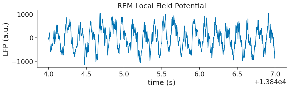
We should first plot our REM Local Field Potential data.
fig, ax = plt.subplots(1, constrained_layout=True, figsize=(10, 3))
ax.plot(tsd_rem.restrict(ep_ex_rem))
ax.set_title("REM Local Field Potential")
ax.set_ylabel("LFP (a.u.)")
ax.set_xlabel("time (s)")
plt.show()
Getting the Wavelet Decomposition#
As we would expect, it looks like we have a very strong theta oscillation within our data
this is a common feature of REM sleep. Let’s perform a wavelet decomposition, as we did in the last tutorial, to see get a more informative breakdown of the frequencies present in the data.
We must define the frequency set that we’d like to use for our decomposition.
freqs = np.geomspace(5, 200, 25)
We compute the wavelet transform on our LFP data (only during the example interval).
cwt_rem = nap.compute_wavelet_transform(tsd_rem.restrict(ep_ex_rem), fs=FS, freqs=freqs)
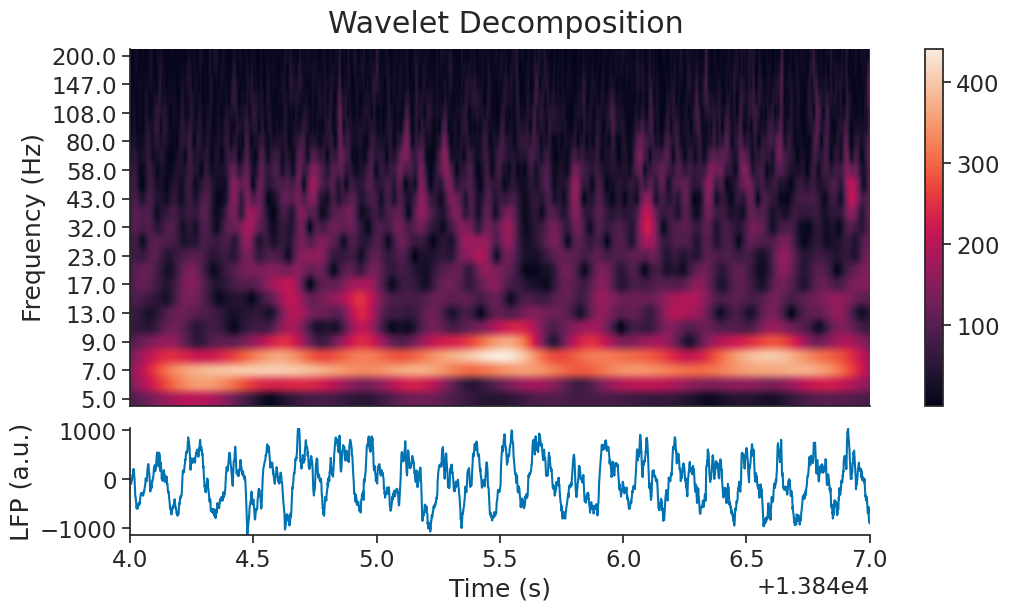
Now let’s plot the calculated wavelet scalogram.
# Define wavelet decomposition plotting function
def plot_timefrequency(freqs, powers, ax=None):
    im = ax.imshow(np.abs(powers), aspect="auto")
    ax.invert_yaxis()
    ax.set_xlabel("Time (s)")
    ax.set_ylabel("Frequency (Hz)")
    ax.get_xaxis().set_visible(False)
    ax.set(yticks=np.arange(len(freqs))[::2], yticklabels=np.rint(freqs[::2]))
    ax.grid(False)
    return im

fig = plt.figure(constrained_layout=True, figsize=(10, 6))
fig.suptitle("Wavelet Decomposition")
gs = plt.GridSpec(2, 1, figure=fig, height_ratios=[1.0, 0.3])

ax0 = plt.subplot(gs[0, 0])
im = plot_timefrequency(freqs, np.transpose(cwt_rem[:, :].values), ax=ax0)
cbar = fig.colorbar(im, ax=ax0, orientation="vertical")

ax1 = plt.subplot(gs[1, 0])
ax1.plot(tsd_rem.restrict(ep_ex_rem))
ax1.set_ylabel("LFP (a.u.)")
ax1.set_xlabel("Time (s)")
ax1.margins(0)
plt.show()
Filtering Theta#
As expected, there is a strong 8Hz component during REM sleep. We can filter it using the function nap.apply_bandpass_filter.
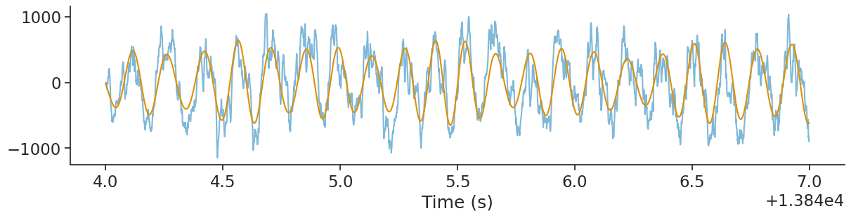
theta_band = nap.apply_bandpass_filter(tsd_rem, cutoff=(6.0, 10.0), fs=FS)
We can plot the original signal and the filtered signal.
plt.figure(constrained_layout=True, figsize=(12, 3))
plt.plot(tsd_rem.restrict(ep_ex_rem), alpha=0.5)
plt.plot(theta_band.restrict(ep_ex_rem))
plt.xlabel("Time (s)")
plt.show()
Computing phase#
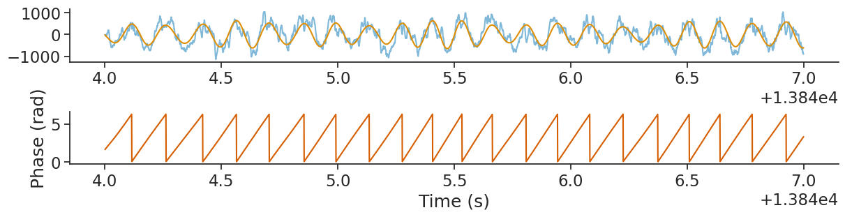
From the filtered signal, it is easy to get the phase using the Hilbert transform, (see the user guide).
Pynapple provides function compute_hilbert_phase for this:
theta_phase = nap.compute_hilbert_phase(theta_band)
theta_phase
Time (s)
----------  --------
13747.0     6.1595
13747.0008  0.597664
13747.0016  0.686686
13747.0024  0.901279
13747.0032  0.973929
13747.004   1.09601
13747.0048  1.16411
...
22572.9952  1.5708
22572.996   1.5708
22572.9968  1.5708
22572.9976  1.5708
22572.9984  1.5708
22572.9992  1.5708
22573.0     4.71239
dtype: float64, shape: (557504,)
Let’s plot the phase.
plt.figure(constrained_layout=True, figsize=(12, 3))
plt.subplot(211)
plt.plot(tsd_rem.restrict(ep_ex_rem), alpha=0.5)
plt.plot(theta_band.restrict(ep_ex_rem))
plt.subplot(212)
plt.plot(theta_phase.restrict(ep_ex_rem), color='r')
plt.ylabel("Phase (rad)")
plt.xlabel("Time (s)")
plt.show()
Finding Phase of Spikes#
Now that we have the phase of our theta wavelet, and our spike times, we can find the phase firing preferences
of each of the units using the compute_tuning_curves function.
We will start by throwing away cells which do not have a high enough firing rate during our interval.
spikes = spikes[spikes.rate > 5.0]
The feature is the theta phase during REM sleep.
phase_modulation = nap.compute_tuning_curves(
    data=spikes,
    features=theta_phase,
    bins=61,
    range=(-np.pi, np.pi),
    feature_names=["Phase"]
)
Let’s plot the first 3 neurons.
phase_modulation.name="Firing Rate"
phase_modulation.attrs["units"]="Hz"
phase_modulation.coords["Phase"].attrs["unit"]="rad"
phase_modulation[:3].plot(row="unit", col_wrap=3, sharey=False)
plt.show()
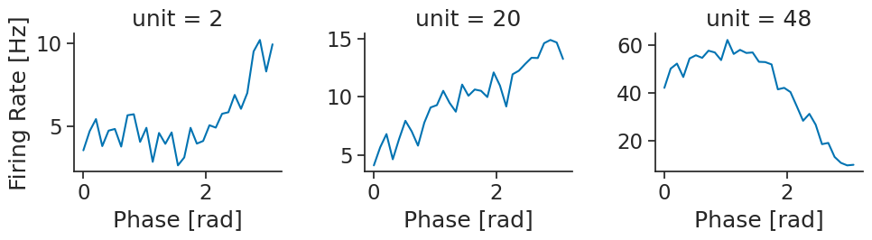
There is clearly a strong modulation for the third neuron.
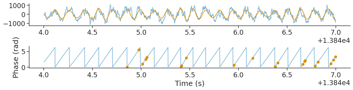
Finally, we can use the function value_from to align each spikes to the corresponding phase position and overlay
it with the LFP.
spike_phase = spikes[spikes.index[3]].value_from(theta_phase)
Let’s plot it.
plt.figure(constrained_layout=True, figsize=(12, 3))
plt.subplot(211)
plt.plot(tsd_rem.restrict(ep_ex_rem), alpha=0.5)
plt.plot(theta_band.restrict(ep_ex_rem))
plt.subplot(212)
plt.plot(theta_phase.restrict(ep_ex_rem), alpha=0.5)
plt.plot(spike_phase.restrict(ep_ex_rem), 'o')
plt.ylabel("Phase (rad)")
plt.xlabel("Time (s)")
plt.show()
Authors
Guillaume Viejo