Trial-aligned decoding with International Brain Lab data#
This example works through a basic pipeline for decoding the mouse’s choice from spiking activity in the International Brain Lab’s decision task, including loading the data from DANDI, processing and trial-aligning the neural activity, and fitting a logistic regression with cross-validation using scikit-learn.
The International Brain Lab’s Brain Wide Map dataset is available at Dandiset 00409. The International Brain Lab’s BWM website includes links to their preprint and additional documentation. The IBL also has an excellent decoding demonstration in the COSYNE section of their events webpage under “Tutorial 2: Advanced analysis”, along with many other relevant demos.
For a more detailed tutorial on data loading with DANDI, see the “Streaming data from DANDI” example!
Caveats: This example is meant to provide a simple starting point for working with trial-aligned data and data from the IBL, and so it does not faithfully replicate the IBL’s quality control and filtering criteria; the decoding here is also simpler than the analyses carried out in those works.
Loading data#
See also the “Streaming data from DANDI”, which includes more detail.
# These modules are used for data loading
from dandi.dandiapi import DandiAPIClient
import fsspec
from fsspec.implementations.cached import CachingFileSystem
import h5py
from pynwb import NWBHDF5IO
# The BWM dandiset:
dandiset_id = "000409"
# This is a randomly chosen recording session.
asset_path = "sub-CSH-ZAD-026/sub-CSH-ZAD-026_ses-15763234-d21e-491f-a01b-1238eb96d389_desc-processed_behavior+ecephys.nwb"
with DandiAPIClient() as client:
    asset = client.get_dandiset(dandiset_id, "draft").get_asset_by_path(asset_path)
    s3_url = asset.get_content_url(follow_redirects=1, strip_query=True)
fs = CachingFileSystem(
    fs=fsspec.filesystem("http"),
    cache_storage=str(Path("~/.caches/nwb-cache").expanduser()),
)
io = NWBHDF5IO(file=h5py.File(fs.open(s3_url, "rb")), load_namespaces=True)
nwb = nap.NWBFile(io.read())
/home/runner/.local/lib/python3.12/site-packages/hdmf/spec/namespace.py:620: UserWarning: Ignoring the following cached namespace(s) because another version is already loaded:
hdmf-common - cached version: 1.9.0, loaded version: 1.8.0
hdmf-experimental - cached version: 0.6.0, loaded version: 0.5.0
Please update to the latest package versions.
  self.warn_for_ignored_namespaces(ignored_namespaces)
This NWB file, loaded into a pynapple object, contains neural activity, behavioral data, and raw electrophysiological traces. They’re lazily loaded, so only what we use will be downloaded.
nwb
15763234-d21e-491f-a01b-1238eb96d389
┍━━━━━━━━━━━━━━━━━━━━━━━━━━━━━━━━━━━━━━┯━━━━━━━━━━━━━┑
│ Keys                                 │ Type        │
┝━━━━━━━━━━━━━━━━━━━━━━━━━━━━━━━━━━━━━━┿━━━━━━━━━━━━━┥
│ units                                │ TsGroup     │
│ trials                               │ IntervalSet │
│ epochs                               │ IntervalSet │
│ WheelMovementIntervals               │ IntervalSet │
│ WheelVelocitySmoothed                │ Tsd         │
│ WheelPositionSmoothed                │ Tsd         │
│ WheelPosition                        │ Tsd         │
│ WheelAccelerationSmoothed            │ Tsd         │
│ RightPupilDiameterSmoothed           │ Tsd         │
│ RightPupilDiameter                   │ Tsd         │
│ PoseEstimationSeriesTubeTop          │ TsdFrame    │
│ PoseEstimationSeriesTubeBottom       │ TsdFrame    │
│ PoseEstimationSeriesRightTongueEnd   │ TsdFrame    │
│ PoseEstimationSeriesRightPupilTop    │ TsdFrame    │
│ PoseEstimationSeriesRightPupilRight  │ TsdFrame    │
│ PoseEstimationSeriesRightPupilLeft   │ TsdFrame    │
│ PoseEstimationSeriesRightPupilBottom │ TsdFrame    │
│ PoseEstimationSeriesRightPaw         │ TsdFrame    │
│ PoseEstimationSeriesNoseTip          │ TsdFrame    │
│ PoseEstimationSeriesLeftTongueEnd    │ TsdFrame    │
│ PoseEstimationSeriesLeftPaw          │ TsdFrame    │
│ PoseEstimationSeriesTailStart        │ TsdFrame    │
│ passive_task_replay                  │ IntervalSet │
│ passive_intervals                    │ IntervalSet │
│ gabor_table                          │ IntervalSet │
│ RightCameraMotionEnergy              │ Tsd         │
│ BodyCameraMotionEnergy               │ Tsd         │
┕━━━━━━━━━━━━━━━━━━━━━━━━━━━━━━━━━━━━━━┷━━━━━━━━━━━━━┙
The only fields we’ll use here are the neural activity (‘units’) and the trial information (‘trials’).
spikes = nwb['units']
trials = nwb['trials']
spikes
Index    rate      unit_name    noise_cutoff    spike_amplitude_std_dB    firing_rate    max_spike_amplitude_uV    spike_count    ...
-------  --------  -----------  --------------  ------------------------  -------------  ------------------------  -------------  -----
0        0.82357   probe00_0    -0.42           1.36                      0.82           562.12                    5079           ...
1        10.99946  probe00_1    259.91          1.54                      11.0           321.68                    67834          ...
2        15.07013  probe00_2    204.26          1.46                      15.07          121.67                    92938          ...
3        5.16569   probe00_3    148.37          1.24                      5.17           135.71                    31857          ...
4        25.96824  probe00_4    44.18           1.47                      25.97          239.12                    160147         ...
5        5.13391   probe00_5    311.32          1.47                      5.13           229.67                    31661          ...
6        15.9644   probe00_6    242.57          1.38                      15.96          227.14                    98453          ...
...      ...       ...          ...             ...                       ...            ...                       ...            ...
903      2.0428    probe00_903  15.81           1.49                      2.04           123.44                    12598          ...
904      0.09989   probe00_904  -0.73           1.48                      0.1            139.46                    616            ...
905      0.16069   probe00_905  -0.85           1.09                      0.16           111.41                    991            ...
906      0.17091   probe00_906  -1.15           1.43                      0.17           82.67                     1054           ...
907      0.05351   probe00_907  4.93            1.37                      0.05           128.79                    330            ...
908      0.05351   probe00_908  -1.5            2.74                      0.05           95.75                     330            ...
909      0.1041    probe00_909  -0.94           1.11                      0.1            164.79                    642            ...
trials
index    start               end                 quiescence_period    gabor_stimulus_onset_time    auditory_cue_time    wheel_movement_onset_time    choice_registration_time    feedback_time    ...
0        36.78385458003678   40.00796416500283   0.46                 37.69                        37.69                37.92                        38.44                       38.44            ...
1        40.375662030040374  43.274770521897445  0.46                 41.39                        41.39                41.59                        41.71                       41.71            ...
2        43.63566933004363   46.29286848474127   0.68                 44.39                        44.39                44.54                        44.71                       44.71            ...
3        46.66926594004667   49.19097904051037   0.61                 47.36                        47.36                47.51                        47.61                       47.61            ...
4        49.55207763004955   55.159877451291685  0.49                 50.11                        50.11                53.28                        53.59                       53.59            ...
5        55.57487529005557   60.826513102388404  0.6                  56.26                        56.26                58.9                         59.25                       59.25            ...
6        61.19131359006119   66.74272338272365   0.62                 61.89                        61.89                65.03                        65.17                       65.17            ...
...      ...                 ...                 ...                  ...                          ...                  ...                          ...                         ...              ...
887      4665.141205894665   4674.910151902795   0.43                 4665.63                      4665.63              4672.21                      4672.34                     4672.34          ...
888      4675.984954744676   4690.743070590566   0.68                 4676.88                      4676.88              4688.64                      4689.19                     4689.19          ...
889      4691.834669614692   4701.794999597876   0.61                 4693.23                      4693.23              4698.98                      4699.21                     4699.21          ...
890      4702.867999504703   4765.977571353986   0.53                 4703.48                      4703.48              nan                          4763.48                     4763.48          ...
891      4767.1222734347675  4830.178418569625   0.48                 4767.68                      4767.68              4820.2                       4827.68                     4827.68          ...
892      4831.3349181948315  4834.507429035308   0.64                 4832.02                      4832.03              4832.64                      4832.96                     4832.96          ...
893      4835.563328644836   4845.873856126055   0.59                 4836.19                      4836.19              4843.87                      4844.31                     4844.31          ...
shape: (894, 2), time unit: sec.
Trial alignment and binning#
Here, we start by discarding some trials where a choice wasn’t made (a more complete analysis may include more criteria).
valid_choice = trials.mouse_wheel_choice != "none"
trials = trials[valid_choice]
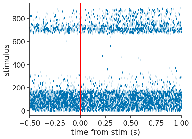
Now, we can use compute_perievent to align the spikes to the
stimulus onset times.
We will choose a window around each stimulus that extends back 0.5s and forward 1s.
stimulus_onsets = nap.Ts(t=trials.gabor_stimulus_onset_time.values)
window=(-0.5, 1.0)
trial_aligned_spikes = nap.compute_perievent(data=spikes, events=stimulus_onsets, window=window)
The result is a dictionary of TsGroup, one per unit, containing that unit’s spikes relative to the onset time.
We can easily visualize that as follows:
example_unit = 42
plt.plot(trial_aligned_spikes[example_unit].to_tsd(), "|", markersize=5)
plt.xlabel("time from stim (s)")
plt.ylabel("stimulus")
plt.xlim(*window)
plt.axvline(0.0, color="red");
Note
See the perievent user guide for how this works and other visualizations!
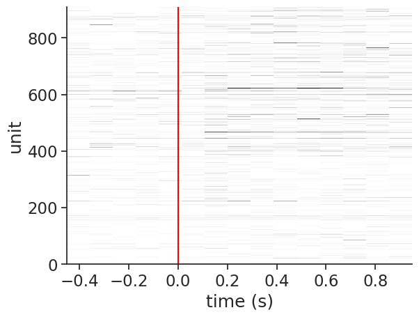
We can then bin and count these spikes as follows:
bin_size = 0.1
trial_aligned_binned_spikes = np.stack([trial_aligned_spikes[unit].count(bin_size) for unit in spikes], axis=1)
trial_aligned_binned_spikes.shape
(15, 910, 892)
Let’s visualize the neural activity in a single trial:
example_trial = 42
plt.imshow(
    trial_aligned_binned_spikes[:, :, example_trial].values.T,
    aspect="auto",
    cmap="Grays",
    interpolation="none",
    extent=(
        trial_aligned_binned_spikes.times()[0],
        trial_aligned_binned_spikes.times()[-1],
        0,
        trial_aligned_binned_spikes.shape[1],
    ),
)
plt.axvline(0, color='red')
plt.ylabel('unit')
plt.xlabel('time (s)');
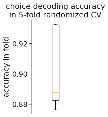
Decoding choice#
Let’s use scikit-learn to fit a logistic regression. We can use their cross-validation tools to pick the regularization parameter
# process the choice from -1, 1 to 0,1
y = (trials.mouse_wheel_choice == "clockwise").astype(int)
# transpose the data to lead with trial dimension
X = trial_aligned_binned_spikes.swapaxes(0, 2)
# standardize per neuron + trial
X = (X - X.mean(2, keepdims=True)) / X.std(2, keepdims=True).clip(min=1e-6)
# reshape to n_trials x n_features
X = X.reshape(len(X), -1)
# loguniform randomized search CV logistic regression
clf = RandomizedSearchCV(
    LogisticRegression(),
    param_distributions={'C': scipy.stats.loguniform(1e-3, 1e3)},
    random_state=0,
)
clf.fit(X, y);
cv_df = pd.DataFrame(clf.cv_results_)
best_row = cv_df[cv_df.rank_test_score == 1]
best_row = best_row.iloc[best_row.param_C.argmin()]
plt.figure(figsize=(2, 4))
plt.boxplot(best_row[[c for c in best_row.keys() if c.startswith('split')]])
plt.ylabel('accuracy in fold')
plt.xticks([])
plt.title("choice decoding accuracy\nin 5-fold randomized CV");
Authors
Charlie Windolf