Streaming data from DANDI

This script shows how to stream data from the DANDI Archive all the way to pynapple.

---

Prelude

The data used in this tutorial were used in this publication: Sargolini, Francesca, et al. “Conjunctive representation of position, direction, and velocity in entorhinal cortex.” Science 312.5774 (2006): 758-762. The data can be found on the DANDI Archive in Dandiset 000582.

---

DANDI

DANDI allows you to stream data without downloading all the files. In this case the data extracted from the NWB file are stored in the nwb-cache folder.

from pynwb import NWBHDF5IO

from dandi.dandiapi import DandiAPIClient
import fsspec
from fsspec.implementations.cached import CachingFileSystem
import h5py


# ecephys
dandiset_id, filepath = (
    "000582",
    "sub-10073/sub-10073_ses-17010302_behavior+ecephys.nwb",
)


with DandiAPIClient() as client:
    asset = client.get_dandiset(dandiset_id, "draft").get_asset_by_path(filepath)
    s3_url = asset.get_content_url(follow_redirects=1, strip_query=True)

# first, create a virtual filesystem based on the http protocol
fs = fsspec.filesystem("http")

# create a cache to save downloaded data to disk (optional)
fs = CachingFileSystem(
    fs=fs,
    cache_storage="nwb-cache",  # Local folder for the cache
)

# next, open the file
file = h5py.File(fs.open(s3_url, "rb"))
io = NWBHDF5IO(file=file, load_namespaces=True)
io

<pynwb.NWBHDF5IO at 0x7ff55f51c500>

Pynapple

If opening the NWB works, you can start streaming data straight into pynapple with the NWBFile class.

import pynapple as nap
import matplotlib.pyplot as plt
import seaborn as sns
import numpy as np

custom_params = {"axes.spines.right": False, "axes.spines.top": False}
sns.set_theme(style="ticks", palette="colorblind", font_scale=1.5, rc=custom_params)

nwb = nap.NWBFile(io.read())
nwb

17010302
┍━━━━━━━━━━━━━━━━━━━━━┯━━━━━━━━━━┑
│ Keys                │ Type     │
┝━━━━━━━━━━━━━━━━━━━━━┿━━━━━━━━━━┥
│ units               │ TsGroup  │
│ ElectricalSeriesLFP │ Tsd      │
│ SpatialSeriesLED1   │ TsdFrame │
│ ElectricalSeries    │ Tsd      │
┕━━━━━━━━━━━━━━━━━━━━━┷━━━━━━━━━━┙

We can load the spikes as a TsGroup for inspection.

units = nwb["units"]
units

  Index     rate  unit_name    histology    hemisphere      depth
-------  -------  -----------  -----------  ------------  -------
      0  2.93217  t1c1         MEC LII                          0
      1  1.50193  t2c1         MEC LII                          0
      2  2.57878  t2c3         MEC LII                          0
      3  1.13186  t3c1         MEC LII                          0
      4  1.29356  t3c2         MEC LII                          0
      5  1.35857  t3c3         MEC LII                          0
      6  2.8855   t3c4         MEC LII                          0
      7  1.46525  t4c1         MEC LII                          0

As well as the position:

position = nwb["SpatialSeriesLED1"]

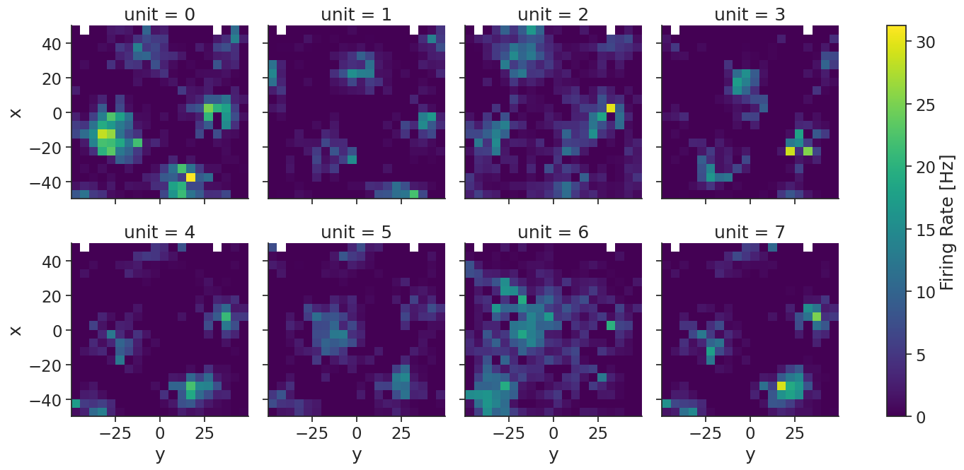
Here, we compute the 2d tuning curves:

tuning_curves = nap.compute_tuning_curves(units, position, 20)

Let’s plot the tuning curves:

tuning_curves.name="Firing Rate"
tuning_curves.attrs["units"] = "Hz"
tuning_curves.plot(row="unit", col_wrap=4, figsize=(15, 7))
plt.show()

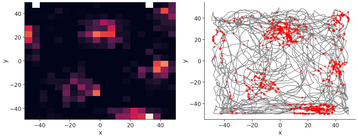
Let’s plot the spikes of unit 1, which has a nice grid. Here, I use the value_from function to assign to each spike the closest position in time.

plt.figure(figsize=(15, 6))
plt.subplot(121)
extent = (
    np.min(position["x"]),
    np.max(position["x"]),
    np.min(position["y"]),
    np.max(position["y"]),
)
plt.imshow(tuning_curves[1], origin="lower", extent=extent, aspect="auto")
plt.xlabel("x")
plt.ylabel("y")

plt.subplot(122)
plt.plot(position["y"], position["x"], color="grey")
spk_pos = units[1].value_from(position)
plt.plot(spk_pos["y"], spk_pos["x"], "o", color="red", markersize=5, alpha=0.5)
plt.xlabel("x")
plt.ylabel("y")
plt.tight_layout()
plt.show()