Null distributions to test spatial firing#
Null distributions are ubiquitous in neuroscience. The brain can be incredibly noisy, and thus we need to use adequate statistical quantification to separate meaningful observations from random fluctuations. While statistics can be daunting, most often designing the right statistical test comes down to devising a good null distribution. A null distribution should reflect the expected behavior of the system under the assumption of no real effect, without introducing unnecessary assumptions or simplifications. We can then compare our observations to such a null distribution to decide whether there is an effect.
If you want to learn the in’s and out’s of statistical analysis of neural data, we’d advise picking up a book about it!
In this tutorial, we will use Pynapple’s randomization module to generate various null distributions to test whether the activity of neurons is modulated by position.
Downloading data from DANDI#
We will start by downloading some data off of DANDI.
To do so, we need a dandiset ID, and a file path.
In this tutorial we will use data from dandiset 000582, which was published in:
Sargolini, Francesca, et al. “Conjunctive representation of position, direction, and velocity in entorhinal cortex.” Science 312.5774 (2006): 758-762
This dataset contains electrophysiology recordings from neurons in the entorhinal cortex, which are known to modulate their firing with position.
dandiset = "000582"
session = "sub-10884/sub-10884_ses-03080402_behavior+ecephys.nwb"

with DandiAPIClient() as client:
    asset = client.get_dandiset(dandiset, "draft").get_asset_by_path(session)
    s3_url = asset.get_content_url(follow_redirects=1, strip_query=True)
fs = CachingFileSystem(
    fs=fsspec.filesystem("http"),
    cache_storage=str(Path("~/.caches/nwb-cache").expanduser()),
)
io = NWBHDF5IO(file=h5py.File(fs.open(s3_url, "rb")), load_namespaces=True)
nwb = nap.NWBFile(io.read(), lazy_loading=False)

units = nwb["units"]
position = nwb["SpatialSeriesLED1"]
Spatial tuning curves#
We can then use compute_tuning_curves to compute the tuning curve for each neuron’s spikes with respect to the position of the animal:
tuning_curves = nap.compute_tuning_curves(
    data=units,
    features=position,
    feature_names=["X", "Y"],
    range=[(-50, 50), (-50, 50)],
    bins=40,
)

# optional smoothing of tuning curves
def gaussian_filter_nan(a, sigma):
    v = np.where(np.isnan(a), 0, a)
    w = gaussian_filter((~np.isnan(a)).astype(float), sigma)
    return gaussian_filter(v, sigma) / w
tuning_curves_smooth = tuning_curves.copy()
tuning_curves_smooth.values = gaussian_filter_nan(tuning_curves.values, sigma=(0, 2, 2))

# Setting some xarray.DataArray attributes, for beauty
tuning_curves_smooth.name = "firing rate"
tuning_curves_smooth.attrs["unit"] = "Hz"
tuning_curves_smooth.coords["X"].attrs["unit"] = "cm"
tuning_curves_smooth.coords["Y"].attrs["unit"] = "cm"
tuning_curves
<xarray.DataArray (unit: 6, X: 40, Y: 40)> Size: 77kB
array([[[ 2.94117647,  0.        ,         nan, ...,  0.        ,
          0.        ,  1.38888889],
        [ 4.54545455,  0.        ,  7.89473684, ...,         nan,
                 nan,  0.        ],
        [ 0.        ,  0.        ,         nan, ...,         nan,
                 nan,  0.        ],
        ...,
        [ 0.        ,  0.        ,  0.        , ...,  0.        ,
          0.        ,  0.94339623],
        [ 0.        ,  4.16666667,  0.        , ...,  0.        ,
          0.        ,  2.7173913 ],
        [ 0.        ,  4.54545455,  0.        , ...,  4.54545455,
          0.90909091,  1.5625    ]],

       [[ 0.        ,  2.94117647,         nan, ...,  0.        ,
          0.        ,  0.        ],
        [ 0.        ,  0.52083333,  0.        , ...,         nan,
                 nan,  0.        ],
        [ 0.        ,  0.        ,         nan, ...,         nan,
                 nan,  0.        ],
...
        [ 0.        ,  0.        ,  8.33333333, ...,  7.44680851,
          5.        ,  3.4591195 ],
        [ 6.25      ,  0.        ,  0.92592593, ..., 12.06896552,
          3.48837209,  4.89130435],
        [ 0.        ,  0.        ,  0.        , ...,  9.09090909,
          4.54545455,  3.90625   ]],

       [[ 2.94117647,  0.        ,         nan, ...,  0.        ,
          0.        ,  2.77777778],
        [ 0.        ,  0.52083333,  0.        , ...,         nan,
                 nan,  0.        ],
        [ 0.        ,  0.        ,         nan, ...,         nan,
                 nan,  0.        ],
        ...,
        [ 0.        ,  0.        ,  0.        , ...,  5.31914894,
          5.        ,  1.88679245],
        [ 6.25      ,  0.        ,  8.33333333, ...,  0.        ,
          0.        ,  0.54347826],
        [ 9.52380952,  6.81818182,  3.84615385, ...,  7.57575758,
          9.09090909, 10.9375    ]]], shape=(6, 40, 40))
Coordinates:
  * unit     (unit) int64 48B 0 1 2 3 4 5
  * X        (X) float64 320B -48.75 -46.25 -43.75 -41.25 ... 43.75 46.25 48.75
  * Y        (Y) float64 320B -48.75 -46.25 -43.75 -41.25 ... 43.75 46.25 48.75
Attributes: (4)We can further also compute our metric of interest. In this case, we are interested in the modulation of the neurons’ firing by position. A metric that is typically used to quantify this is the mutual information, often called spatial information for this case specifically:
spatial_information = nap.compute_mutual_information(tuning_curves)
spatial_information
| bits/sec | bits/spike | |
|---|---|---|
| 0 | 2.797138 | 1.389261 |
| 1 | 2.408331 | 2.670888 |
| 2 | 2.412850 | 3.133467 |
| 3 | 3.301270 | 2.673004 |
| 4 | 1.965672 | 2.290027 |
| 5 | 1.832783 | 2.013981 |
We can visualize all that together:
g = tuning_curves_smooth.plot(col="unit")
for ax, (unit_idx, unit_id) in zip(g.axs.flat, enumerate(units)):
    ax.set_title(f"unit={unit_id}\nSI={spatial_information['bits/spike'][unit_idx]:.2f}")
plt.show()
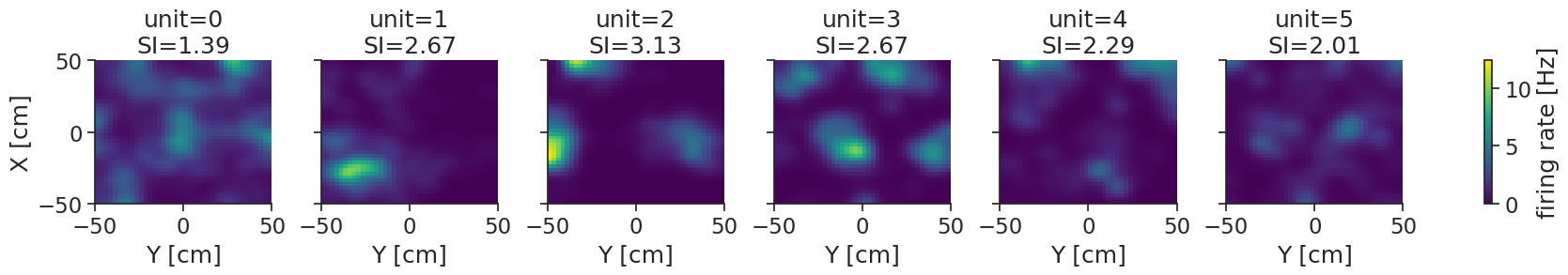
Some of these units seem to have clear spatial firing (e.g. unit 3), with localized firing fields and relatively high spatial information values. However, for units like unit 0 we can not say for certain that the pattern we see is not just caused by random activity.
Randomization#
Next, we can start thinking about null distributions. Our ultimate goal is to be able to say that a neuron’s activity is significantly modulated by position. To do that, we want to contrast it to the activity of a neuron that is not modulated by position at all. But how do we pick that neuron? We do not want to stray away from the firing patterns of our neuron of interest too much, so we can’t just pick something arbitrary.
In practice, we will often take the activity of our neuron of interest and shuffle it somehow, thereby breaking the relation with our variable of interest (position), but keeping its general firing statistics as much as possible.
Pynapple provides four methods for such shuffling:
jitter_timestamps: jitters timestamps independently by random amounts uniformly drawn from a given range.resample_timestamps: uniformly resamples all timestamps within the time support.shift_timestamps: shifts all timestamps by a random amount drawn from a given range:mode='drop': dropping spikes that fall out of the time support.mode='wrap': wrapping the end of the time support to the beginning (we will use this one as it retains most of the data).
shuffle_ts_intervals: randomizes timestamps by shuffling the intervals between them.
Let’s apply them to an example neuron:
jitter = nap.jitter_timestamps(units[3], max_jitter=2.0)
resample = nap.resample_timestamps(units[3])
shift = nap.shift_timestamps(units[3], min_shift=10.0, mode="wrap")
interval_shuffle = nap.shuffle_ts_intervals(units[3])
and plot them to look at their effect on spatial firing:
fig, axs = plt.subplots(3, 5, figsize=(10, 6))
for (ax_spikes, ax_tc, ax_corr), (randomization_type, data) in zip(
    axs.T,
    [
        ("true", units[3]),
        ("jitter", jitter),
        ("resample", resample),
        ("shift", shift),
        ("interval_shuffle", interval_shuffle),
    ],
):
    # Plot spike positions
    ax_spikes.plot(position[:, 0], position[:, 1], color="black", linewidth=0.5, zorder=-1)
    positional_spikes = data.value_from(position)
    ax_spikes.scatter(
        positional_spikes[:, 1],
        positional_spikes[:, 0],
        color="red",
        s=7,
        edgecolor="none",
        zorder=1
    )
    ax_spikes.yaxis.set_inverted(True)
    ax_spikes.axis("off")
    ax_spikes.set_title(randomization_type.replace("_", "\n"))

    # Plot tuning curve
    tuning_curve = nap.compute_tuning_curves(
        data,
        features=position,
        feature_names=["X", "Y"],
        range=[(-50, 50), (-50, 50)],
        bins=40
    )
    tuning_curve.values = gaussian_filter_nan(tuning_curve.values, sigma=(0, 2, 2))
    ax_tc.imshow(tuning_curve.values[0], cmap="viridis", extent=(-50, 50, -50, 50))
    ax_tc.axis("off")

    # Plot 2D autocorrelation
    ax_corr.imshow(correlate2d(tuning_curve[0], tuning_curve[0]), cmap="viridis")
    ax_corr.axis("off")
fig.text(0.09, 0.44, "tuning\ncurve", rotation=90, ha="center")
fig.text(0.09, 0.12, "auto\ncorrelation", rotation=90, ha="center")
plt.show()
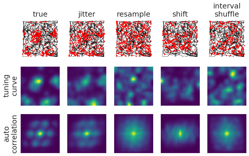
We are also visualizing the two-dimensional autocorrelation of the tuning curves here to highlight the breaking/maintaining of patterns.
Each of these methods seem to have different effects:
Jittering: does exactly that, the jitter in time also results in a jitter in position. We set the maximal jitter to 2 seconds, which likely matches the timescale of the movements of the animal. The tuning curve and autocorrelation have not changed a lot, meaning we have not broken the relation between spiking and behavior. Thus, jittering might not be a good randomization method in this case, unless we increase the maximal jitter.
Resampling: gives us a uniform spread in position, the relation between spiking and behaviour is gone entirely.
Shifting: has the advantage of keeping the temporal relations between spikes, while only breaking the relation with position.
Shuffling interspike intervals: looks similar to shifting, it keeps the overall interspike interval distribution.
Null distributions#
We will opt for random shifts.
For each neuron, we will generate N pseudo-neurons and compute the mutual/spatial information.
The resulting distributions of values are what we call the null distributions.
N = 500
shuffles = [nap.shift_timestamps(units, min_shift=20.0, mode="wrap") for _ in range(N)]

null_distributions = np.stack(
    [
        nap.compute_mutual_information(
            nap.compute_tuning_curves(
                data=shuffle,
                features=position,
                range=[(-50, 50), (-50, 50)],
                bins=40,
            )
        )["bits/spike"].values
        for shuffle in shuffles
    ],
    axis=1,
)
null_distributions.shape
(6, 500)
Testing#
Ultimately, we will apply the test. From a statistical view, we see the null distribution as an empirical distribution of spatial information values that would be expected if the neuron’s firing were unrelated to spatial position. We want to determine how unlikely it is that the observed spatial information arose from our null distribution.
Given a significance level, α, we assess whether the observed value lies in the extreme tail of the null distribution. If the probability (the p-value) of obtaining a spatial information value as large as or larger than the observed one is less than α, we reject the null hypothesis:
alpha = 0.01 # significance level
p_values = np.sum(
    null_distributions.T >= spatial_information['bits/spike'].values,
    axis=0
    ) / null_distributions.shape[1]
spatial_units = tuning_curves.coords["unit"][p_values < alpha]
We can further also compute the exact spatial information values corresponding to our alpha:
thresholds = np.nanpercentile(null_distributions, (1-alpha)*100, axis=1)
Finally, we can visualize everything together:
g = tuning_curves_smooth.plot(col="unit")
for ax, (unit_idx, unit_id) in zip(g.axs.flat, enumerate(units)):
    null = null_distributions[unit_idx]
    score = spatial_information['bits/spike'][unit_idx]
    pval = p_values[unit_idx]

    ax.set_title(f"unit={unit_id}\nSI={score:.2f}\np={pval:.6f}{'*' if score>thresholds[unit_idx] else ''}")

    ax_hist = inset_axes(ax, width="100%", height="40%", loc="lower center",
                         bbox_to_anchor=(0, -1, 1, 1), bbox_transform=ax.transAxes, borderpad=0)

    ax_hist.hist(null, histtype="stepfilled", edgecolor="none", bins=30)
    ax_hist.axvline(thresholds[unit_idx], color="black")
    ax_hist.axvline(score, color="red", linestyle="--")
    ax_hist.yaxis.set_visible(False)
    ax_hist.spines['left'].set_visible(False)
    if unit_idx == 0:
        ax_hist.set_xlabel("spatial\ninformation\n(bits/spike)")
plt.show()
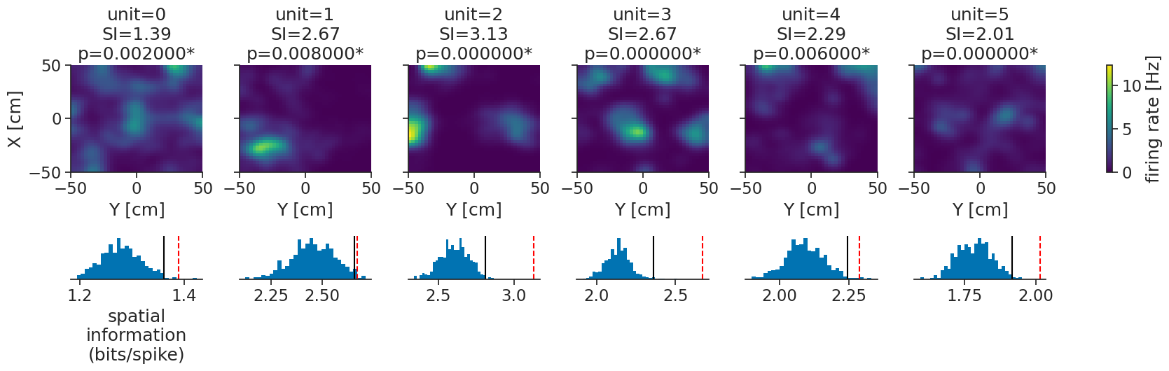
We can see that all our units are significantly modulated by position, some more so than others. By visualizing the null distributions (blue histograms), the percentile thresholds (black lines), and the actual values (dashed red lines), we can get more nuance. We now also have approximate p-values to report.
Authors