Detecting sharp-wave ripples

This tutorial demonstrates how to use Pynapple to detect sharp-wave ripples.

Show code cell source

Hide code cell source

# we'll import the packages we're going to use
import math
import os

import matplotlib.colors as mcolors
import matplotlib.pyplot as plt
import numpy as np
import requests
import seaborn as sns
import pynapple as nap

# some configuration, you can ignore this
custom_params = {"axes.spines.right": False, "axes.spines.top": False}
sns.set_theme(style="ticks", palette="colorblind", font_scale=1.5, rc=custom_params);

Downloading the data

We will examine the dataset from Grosmark & Buzsáki (2016). Let’s download the data and save it locally:

path = "Achilles_10252013_EEG.nwb"
if path not in os.listdir("."):
    r = requests.get(f"https://osf.io/2dfvp/download", stream=True)
    block_size = 1024 * 1024
    with open(path, "wb") as f:
        for data in r.iter_content(block_size):
            f.write(data)
data = nap.load_file(path)
data

Achilles_10252013_EEG
┍━━━━━━━━━━━━━┯━━━━━━━━━━━━━┑
│ Keys        │ Type        │
┝━━━━━━━━━━━━━┿━━━━━━━━━━━━━┥
│ units       │ TsGroup     │
│ rem         │ IntervalSet │
│ nrem        │ IntervalSet │
│ forward_ep  │ IntervalSet │
│ eeg         │ TsdFrame    │
│ theta_phase │ Tsd         │
│ position    │ Tsd         │
┕━━━━━━━━━━━━━┷━━━━━━━━━━━━━┙

We only need to local field potential (LFP), which has been downsampled to 1250Hz:

lfp = data["eeg"][:, 0]
lfp

Time (s)
----------  ----
12679.5     -258
12679.5008  -341
12679.5016  -355
12679.5024  -379
12679.5032  -364
12679.504   -406
12679.5048  -508
...
25546.9696  2035
25546.9704  2021
25546.9712  2023
25546.972   1906
25546.9728  1848
25546.9736  1862
25546.9744  1976
dtype: int16, shape: (16084344,)

lfp.rate

np.float64(1250.0000777153286)

Frequency filtering

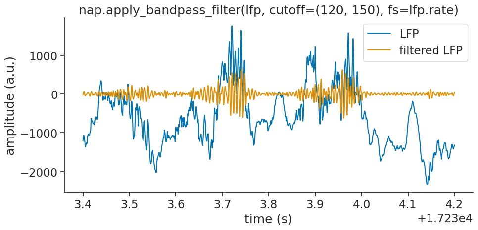
To look for ripples we will only keep frequencies within 120 to 250Hz:

filtered_lfp = nap.apply_bandpass_filter(lfp, cutoff=(120, 250), fs=lfp.rate)
filtered_lfp

Time (s)
----------  ---
12679.5       0
12679.5008  -40
12679.5016  -44
12679.5024  -13
12679.5032   22
12679.504    33
12679.5048   19
...
25546.9696   57
25546.9704   81
25546.9712   49
25546.972   -29
25546.9728  -95
25546.9736  -90
25546.9744  -16
dtype: int16, shape: (16084344,)

Show code cell source

Hide code cell source

segment = nap.IntervalSet(17233.4, 17234.2)
fig = plt.figure(figsize=(10, 5))
plt.plot(lfp.restrict(segment), label="LFP")
plt.plot(filtered_lfp.restrict(segment), label="filtered LFP")
plt.xlabel("time (s)")
plt.ylabel("amplitude (a.u.)")
plt.legend()
plt.title("nap.apply_bandpass_filter(lfp, cutoff=(120, 150), fs=lfp.rate)")
plt.tight_layout();

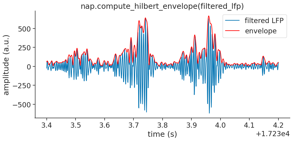
Hilbert transform: computing the envelope

Now, we will apply the Hilbert transform to the filtered LFP and take its absolute value to extract the amplitude envelope, which reflects ripple strength over time. Pynapple provides compute_hilbert_envelope:

envelope = nap.compute_hilbert_envelope(filtered_lfp)
envelope

Time (s)
----------  ---------
12679.5       3.00686
12679.5008   40.3712
12679.5016   54.7394
12679.5024   55.3081
12679.5032   47.6888
12679.504    34.8182
12679.5048   22.0093
...
25546.9696   65.9358
25546.9704   84.1077
25546.9712  101.346
25546.972   110.556
25546.9728  110.843
25546.9736   94.404
25546.9744   51.4788
dtype: float64, shape: (16084344,)

See scipy.signal.hilbert for more information on what the Hilbert transform does!

We will plot the envelope over the filtered signal for visual confirmation:

Show code cell source

Hide code cell source

fig = plt.figure(figsize=(10, 5))
plt.plot(filtered_lfp.restrict(segment), label="filtered LFP")
plt.plot(envelope.restrict(segment), label="envelope", color="red")
plt.xlabel("time (s)")
plt.ylabel("amplitude (a.u.)")
plt.legend()
plt.title("nap.compute_hilbert_envelope(filtered_lfp)")
plt.tight_layout();

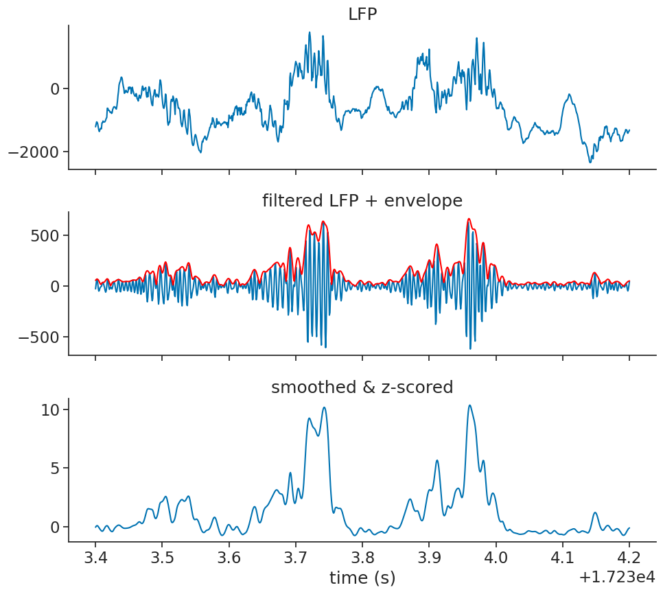
Smooth and Z-score

We will then smooth and z-score the envelope:

smoothing_bins = 10
window = np.ones(smoothing_bins) / smoothing_bins
smoothed = envelope.convolve(window)
zscored_smoothed = (smoothed - smoothed.mean()) / smoothed.std()

Let’s visualize everything up until now as an overview:

Show code cell source

Hide code cell source

fig, axs = plt.subplots(3, 1, figsize=(10,9), sharex=True)
axs[0].plot(lfp.restrict(segment))
axs[0].set_title("LFP")
axs[1].plot(filtered_lfp.restrict(segment))
axs[1].plot(envelope.restrict(segment), color="red")
axs[1].set_title("filtered LFP + envelope")
axs[2].plot(zscored_smoothed.restrict(segment))
axs[2].set_title("smoothed & z-scored")
axs[2].set_xlabel("time (s)")
plt.tight_layout();

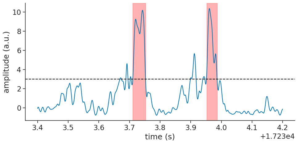
Ripple detection

We detect ripple events by thresholding the z-scored smoothed signal with a threshold of 3 standard deviations. We further filter detected events to keep only those between 30ms and 300ms in duration, typical for hippocampal ripples. We lastly merge events that are closer to each other than 20ms, as they are likely to be the same ripple.

threshold = 3
ripple_events = zscored_smoothed.threshold(threshold, method="above")
ripple_epochs = ripple_events.time_support
ripple_epochs = ripple_epochs.drop_short_intervals(0.03, time_units="s")
ripple_epochs = ripple_epochs.drop_long_intervals(0.3, time_units="s")    
ripple_epochs = ripple_epochs.merge_close_intervals(0.02, time_units="s")
ripple_epochs.intersect(segment)

  index    start      end
      0  17233.7  17233.8
      1  17234    17234
shape: (2, 2), time unit: sec.

Finally, we can plot the detected ripple events on top of the filtered LFP signal for visual confirmation:

Show code cell source

Hide code cell source

fig = plt.figure(figsize=(10, 5))
plt.plot(zscored_smoothed.restrict(segment), label="z-scored & smoothed")
for start, end in ripple_epochs.intersect(segment).values:
    plt.axvspan(start, end, alpha=0.3, color="red")
plt.axhline(threshold, color="black", linestyle="--")
plt.ylabel("amplitude (a.u.)")
plt.xlabel("time (s)")
plt.tight_layout();

Using detect_oscillatory_events

For your convenience, we put the entire process into a single function called detect_oscillatory_events.

To get it to work nicely, you will have to the tune the following detection parameters:

• frequency band: the band of frequencies you are interested in

• threshold band: minimum and maximum thresholds to apply to the z-scored envelope of the squared signal

• duration band: minimum and maximum duration of the events

• minimum interval between events

ripple_epochs = nap.detect_oscillatory_events(
    data=lfp,
    epochs=lfp.time_support,
    frequency_band=(120, 250),
    threshold_band=(3, 15),
    duration_band=(0.03, 0.3),
    min_interval=0.02,
    sliding_window_size=smoothing_bins
)
ripple_epochs.intersect(segment)

  index    start      end    power    amplitude    peak_time
      0  17233.7  17233.8    54.28       641.17      17233.7
      1  17234    17234      53.48       666.65      17234
shape: (2, 2), time unit: sec.

You can see that this gives the same result as before:

Show code cell source

Hide code cell source

fig = plt.figure(figsize=(10, 5))
plt.plot(zscored_smoothed.restrict(segment), label="z-scored & smoothed")
for start, end in ripple_epochs.intersect(segment).values:
    plt.axvspan(start, end, alpha=0.3, color="red")
plt.axhline(threshold, color="black", linestyle="--")
plt.ylabel("amplitude (a.u.)")
plt.xlabel("time (s)")
plt.tight_layout();

Authors

Wolf De Wulf

Guillaume Viejo