Decoding

Show code cell content

Hide code cell content

import pynapple as nap
import numpy as np
import pandas as pd
import matplotlib.pyplot as plt
import seaborn as sns
custom_params = {"axes.spines.right": False, "axes.spines.top": False}
sns.set_theme(style="ticks", palette="colorblind", font_scale=1.5, rc=custom_params)

Pynapple supports n-dimensional decoding from any neural modality. For spike data, you can use decode_bayes, which implements Bayesian decoding using a Poisson distribution. For any other type of data (and also for spike data), you can use decode_template, which implements a template matching algorithm.

Input to both decoding functions always includes:

• tuning_curves, computed using compute_tuning_curves.

• data, neural activity as a TsGroup (spikes) or TsdFrame (smoothed counts or calcium activity or any other time series).

• epochs, to restrict decoding to certain intervals.

• sliding_window_size, uniform convolution window size (in number of bins) to smooth spike counts, only used if a TsGroup is passed (default is None, for no smoothing). This is equivalent to using a sliding window with overlapping bins.

• bin_size, the size of the bins in which to count timestamps when data is a TsGroup object.

• time_units, the units of bin_size, defaulting to seconds.

Bayesian decoding

When using Bayesian decoding, users can additionally set uniform_prior=False to use the occupancy as a prior over the feature distribution. By default uniform_prior=True, and a uniform prior is used.

Important

Bayesian decoding should only be used with spike (TsGroup) or spike count (TsdFrame) data, as these can be assumed to follow a Poisson distribution!

1-dimensional Bayesian decoding

Show code cell content

Hide code cell content

from scipy.ndimage import gaussian_filter1d

# Fake Tuning curves
N = 6 # Number of neurons
bins = np.linspace(0, 2*np.pi, 61)
x = np.linspace(-np.pi, np.pi, len(bins)-1)
tmp = np.roll(np.exp(-(1.5*x)**2), (len(bins)-1)//2)
tc = np.array([np.roll(tmp, i*(len(bins)-1)//N) for i in range(N)]).T

tc_1d = pd.DataFrame(index=bins[0:-1], data=tc)

# Feature
T = 10000
dt = 0.01
timestep = np.arange(0, T)*dt
feature = nap.Tsd(
    t=timestep,
    d=gaussian_filter1d(np.cumsum(np.random.randn(T)*0.5), 20)%(2*np.pi)
    )
index = np.digitize(feature, bins)-1

# Spiking activity

count = np.random.poisson(tc[index])>0
tsgroup = nap.TsGroup({i:nap.Ts(timestep[count[:,i]]) for i in range(N)})
epochs = nap.IntervalSet(0, 10)

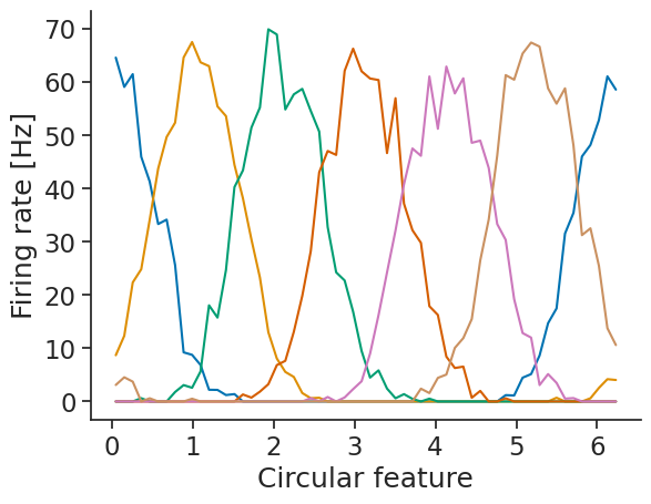
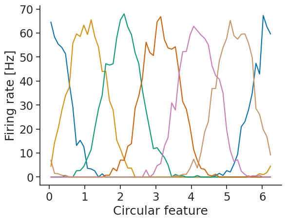
First, we compute the tuning curves:

tuning_curves_1d = nap.compute_tuning_curves(
    tsgroup, 
    feature, 
    bins=60, 
    range=(0, 2 * np.pi), 
    feature_names=["Circular feature"]
)

Show code cell source

Hide code cell source

tuning_curves_1d.name = "Firing rate"
tuning_curves_1d.attrs["unit"] = "Hz"
tuning_curves_1d.plot.line(x="Circular feature", add_legend=False)
plt.show()

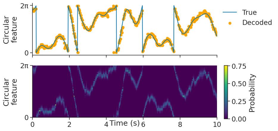
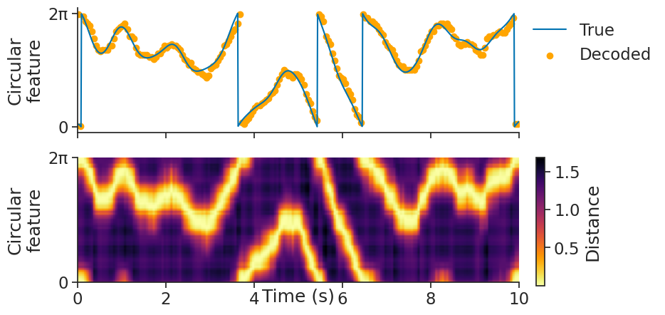
We can then use decode_bayes for Bayesian decoding. We will use the sliding_window_size argument to additionally smooth the spike counts with a uniform convolution window (i.e. use a sliding window), which often helps with decoding.

decoded, proba_feature = nap.decode_bayes(
    tuning_curves=tuning_curves_1d,
    data=tsgroup,
    epochs=epochs,
    sliding_window_size=4,
    bin_size=0.02,
)

decoded is a Tsd object containing the decoded feature value. proba_feature is a TsdFrame containing the probabilities of being in a particular feature bin over time.

Show code cell source

Hide code cell source

fig, (ax1, ax2) = plt.subplots(figsize=(8, 5), nrows=2, ncols=1, sharex=True)
feature=feature.restrict(epochs)
ax1.plot(
    feature.times(),
    feature.values,
    label="True",
)
ax1.scatter(
    decoded.times(),
    decoded.values,
    label="Decoded",
    c="orange",
)
ax1.legend(
    frameon=False,
    bbox_to_anchor=(1.0, 1.0),
)
ax1.set_ylabel("Circular\nfeature")
ax1.set_yticks([0, 2*np.pi], ["0", "2π"])
im = ax2.imshow(proba_feature.values.T, aspect="auto", origin="lower", cmap="viridis", extent=(0, 10.0, 0, 2*np.pi))
cbar_ax = fig.add_axes([0.93, 0.1, 0.015, 0.36])
fig.colorbar(im, cax=cbar_ax, label="Probability")
ax2.set_xlabel("Time (s)", labelpad=-20)
ax2.set_ylabel("Circular\nfeature")
ax2.set_yticks([0, 2*np.pi], ["0", "2π"])
plt.show()

N-dimensional Bayesian decoding

Show code cell content

Hide code cell content

dt = 0.1
epochs = nap.IntervalSet(start=0, end=1000, time_units="s")
features = np.vstack((np.cos(np.arange(0, 1000, dt)), np.sin(np.arange(0, 1000, dt)))).T
features = nap.TsdFrame(
    t=np.arange(0, 1000, dt),
    d=features,
    time_units="s",
    time_support=epochs,
    columns=["a", "b"],
)

times = features.as_units("us").index.values
ft = features.values
alpha = np.arctan2(ft[:, 1], ft[:, 0])
bin_centers = np.linspace(-np.pi, np.pi, 12)
kappa = 4.0
ts_group = {}
for i, mu in enumerate(bin_centers):
    weights = np.exp(kappa * np.cos(alpha - mu))  # wrapped Gaussian
    weights /= np.max(weights)  # normalize to 0–1
    mask = weights > 0.5
    ts = times[mask]
    ts_group[i] = nap.Ts(ts, time_units="us")
ts_group = nap.TsGroup(ts_group)

Decoding also works with multiple dimensions (here we show a 2D example).

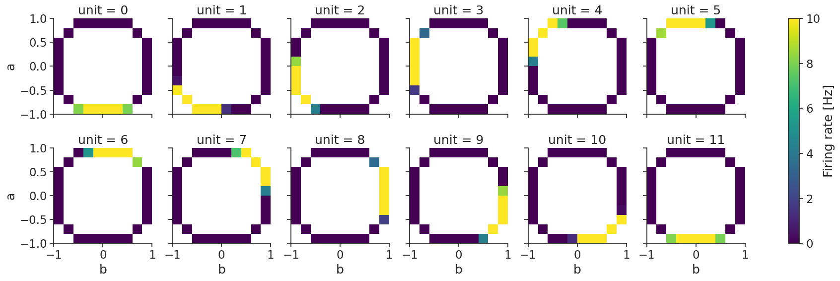
First, we compute the tuning curves:

tuning_curves_2d = nap.compute_tuning_curves(
    data=ts_group,
    features=features, # containing 2 features
    bins=10,
    epochs=epochs,
    range=[(-1.0, 1.0), (-1.0, 1.0)], # range can be specified for each feature
)

Show code cell source

Hide code cell source

tuning_curves_2d.name = "Firing rate"
tuning_curves_2d.attrs["unit"] = "Hz"
tuning_curves_2d.plot(row="unit", col_wrap=6)
plt.show()

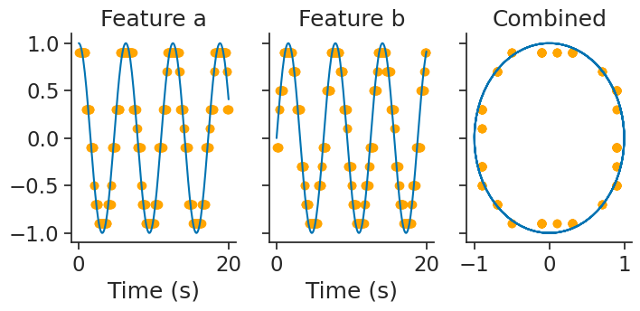
and then, decode_bayes again performs bayesian decoding:

decoded, proba_feature = nap.decode_bayes(
    tuning_curves=tuning_curves_2d,
    data=ts_group,
    epochs=epochs,
    sliding_window_size=2,
    bin_size=0.05,
)

Show code cell source

Hide code cell source

fig, (ax1, ax2, ax3) = plt.subplots(figsize=(8, 3), nrows=1, ncols=3, sharey=True)
ax1.plot(features["a"].get(0, 20), label="True")
ax1.scatter(
    decoded["a"].get(0, 20).times(),
    decoded["a"].get(0, 20),
    label="Decoded",
    c="orange",
)
ax1.set_title("Feature a")
ax1.set_xlabel("Time (s)")

ax2.plot(features["b"].get(0, 20), label="True")
ax2.scatter(
    decoded["b"].get(0, 20).times(),
    decoded["b"].get(0, 20),
    label="Decoded",
    c="orange",
)
ax2.set_xlabel("Time (s)")
ax2.set_title("Feature b")

ax3.plot(
    features["a"].get(0, 20),
    features["b"].get(0, 20),
    label="True",
)
ax3.scatter(
    decoded["a"].get(0, 20),
    decoded["b"].get(0, 20),
    label="Decoded",
    c="orange",
)
ax3.set_title("Combined")
plt.show()

Template matching

If you do not have spike data, or if you do not want to use the Poisson assumption, Pynapple also supports decoding using template matching, which makes no assumption on the modality of your data. Instead of computing a probability distribution, compute_template computes a distance matrix between the samples and the tuning curves (smaller is better). In addition to the default arguments, users can set metric to choose the used distance metric. By default metric="correlation".

1-dimensional template matching

Show code cell content

Hide code cell content

from scipy.ndimage import gaussian_filter1d

# Fake Tuning curves
N = 6 # Number of neurons
bins = np.linspace(0, 2*np.pi, 61)
x = np.linspace(-np.pi, np.pi, len(bins)-1)
tmp = np.roll(np.exp(-(1.5*x)**2), (len(bins)-1)//2)
tc = np.array([np.roll(tmp, i*(len(bins)-1)//N) for i in range(N)]).T

tc_1d = pd.DataFrame(index=bins[0:-1], data=tc)

# Feature
T = 10000
dt = 0.01
timestep = np.arange(0, T)*dt
feature = nap.Tsd(
    t=timestep,
    d=gaussian_filter1d(np.cumsum(np.random.randn(T)*0.5), 20)%(2*np.pi)
    )
index = np.digitize(feature, bins)-1

# Spiking activity

count = np.random.poisson(tc[index])>0
tsgroup = nap.TsGroup({i:nap.Ts(timestep[count[:,i]]) for i in range(N)})
epochs = nap.IntervalSet(0, 10)

First, we compute the tuning curves (here we’ll use spikes as neural data):

tuning_curves_1d = nap.compute_tuning_curves(
    tsgroup, 
    feature, 
    bins=61, 
    range=(0, 2 * np.pi), 
    feature_names=["Circular feature"]
)

Show code cell source

Hide code cell source

tuning_curves_1d.name = "Firing rate"
tuning_curves_1d.attrs["unit"] = "Hz"
tuning_curves_1d.plot.line(x="Circular feature", add_legend=False)
plt.show()

We can then use decode_template for template matching:

decoded, dist = nap.decode_template(
    tuning_curves=tuning_curves_1d,
    data=tsgroup,
    epochs=epochs,
    sliding_window_size=4,
    bin_size=0.05,
    metric="correlation"
)

decoded is a Tsd object containing the decoded feature value. dist is a TsdFrame containing the distance matrix of every time bin with respect to the tuning curves.

Show code cell source

Hide code cell source

fig, (ax1, ax2) = plt.subplots(figsize=(8, 5), nrows=2, ncols=1, sharex=True)
feature=feature.restrict(epochs)
ax1.plot(
    feature.times(),
    feature.values,
    label="True",
)
ax1.scatter(
    decoded.times(),
    decoded.values,
    label="Decoded",
    c="orange",
)
ax1.legend(
    frameon=False,
    bbox_to_anchor=(1.0, 1.0),
)
ax1.set_ylabel("Circular\nfeature")
ax1.set_yticks([0, 2*np.pi], ["0", "2π"])
im = ax2.imshow(dist.values.T, aspect="auto", origin="lower", cmap="inferno_r", extent=(0, 10.0, 0, 2*np.pi))
cbar_ax = fig.add_axes([0.93, 0.1, 0.015, 0.36])
fig.colorbar(im, cax=cbar_ax, label="Distance")
ax2.set_xlabel("Time (s)", labelpad=-20)
ax2.set_ylabel("Circular\nfeature")
ax2.set_yticks([0, 2*np.pi], ["0", "2π"])
plt.show()

N-dimensional template matching

Show code cell content

Hide code cell content

dt = 0.01
T = 10
epoch = nap.IntervalSet(start=0, end=T, time_units="s")
features = np.vstack((np.cos(np.arange(0, T, dt)), np.sin(np.arange(0, T, dt)))).T
features = nap.TsdFrame(
    t=np.arange(0, T, dt),
    d=features,
    time_units="s",
    time_support=epoch,
    columns=["a", "b"],
)


# Calcium activity
ft = features.values
alpha = np.arctan2(ft[:, 1], ft[:, 0])
bin_centers = np.linspace(-np.pi, np.pi, 12)
kappa = 4.0
units=[]
for i, mu in enumerate(bin_centers):
    units.append(np.exp(kappa * np.cos(alpha - mu))) # wrapped Gaussian
units = np.stack(units, axis=1)
tsdframe = nap.TsdFrame(t=features.times(), d=units)

Template matching also works with multiple dimensions.

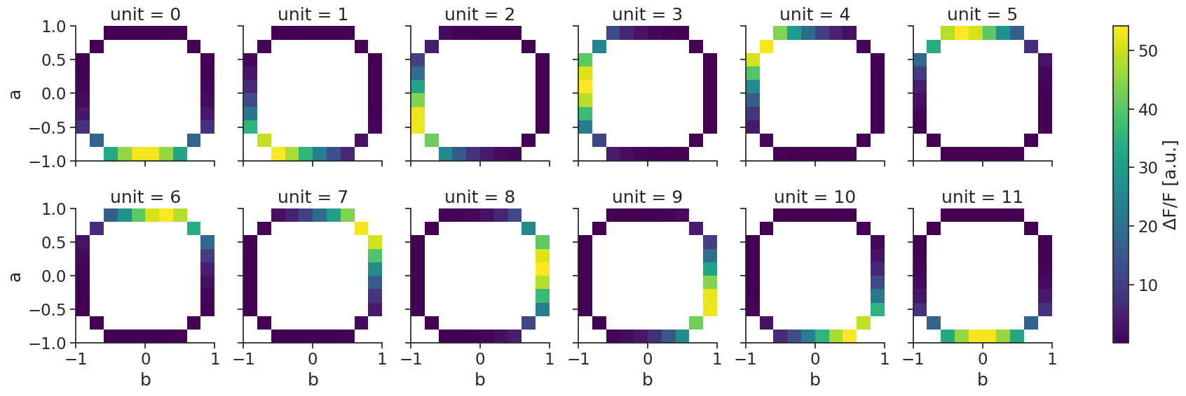
First, we compute the tuning curves (now let’s simulate calcium imaging in a TsdFrame):

tuning_curves_2d = nap.compute_tuning_curves(
    data=tsdframe,
    features=features, # containing 2 features
    bins=10,
    epochs=epochs,
    range=[(-1.0, 1.0), (-1.0, 1.0)], # range can be specified for each feature
)

Show code cell source

Hide code cell source

tuning_curves_2d.name = "ΔF/F"
tuning_curves_2d.attrs["unit"] = "a.u."
tuning_curves_2d.plot(row="unit", col_wrap=6)
plt.show()

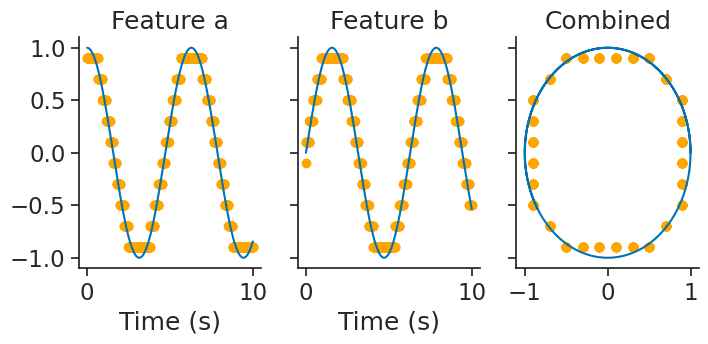
and then, decode_template again performs template matching:

decoded, dist = nap.decode_template(
    tuning_curves=tuning_curves_2d,
    data=tsdframe,
    epochs=epochs,
    bin_size=0.01,
    metric="correlation"
)

Show code cell source

Hide code cell source

fig, (ax1, ax2, ax3) = plt.subplots(figsize=(8, 3), nrows=1, ncols=3, sharey=True)
ax1.plot(features["a"].get(0, 20), label="True")
ax1.scatter(
    decoded["a"].get(0, 20).times(),
    decoded["a"].get(0, 20),
    label="Decoded",
    c="orange",
)
ax1.set_title("Feature a")
ax1.set_xlabel("Time (s)")

ax2.plot(features["b"].get(0, 20), label="True")
ax2.scatter(
    decoded["b"].get(0, 20).times(),
    decoded["b"].get(0, 20),
    label="Decoded",
    c="orange",
)
ax2.set_xlabel("Time (s)")
ax2.set_title("Feature b")

ax3.plot(
    features["a"].get(0, 20),
    features["b"].get(0, 20),
    label="True",
)
ax3.scatter(
    decoded["a"].get(0, 20),
    decoded["b"].get(0, 20),
    label="Decoded",
    c="orange",
)
ax3.set_title("Combined")
plt.show()

Take a look at the tutorial on calcium imaging for an application of template matching with real data and a comparison of various distance metrics!