Input-output & lazy-loading

Pynapple provides multiple ways to load data. The two main formats are NWB and NPZ. In addition, raw data can be loaded through the NEO library.

Each pynapple objects can be saved as a npz with a Pynapple-specific structure and loaded as a npz.

In addition, the Folder class helps you walk through a set of nested folders to load/save npz/nwb files.

NWB

When loading a NWB file, pynapple will walk through it and test the compatibility of each data structure with a pynapple objects. If the data structure is incompatible, pynapple will ignore it. The class that deals with reading NWB file is nap.NWBFile. You can pass the path to a NWB file or directly an opened NWB file. Alternatively you can use the function nap.load_file.

Note

Creating the NWB file is outside the scope of pynapple. The NWB files used here have already been created before. Multiple tools exists to create NWB file automatically. You can check neuroconv, NWBGuide or even NWBmatic.

Show code cell content

Hide code cell content

import numpy as np
import pynapple as nap
import os
import requests, math
import tqdm
import matplotlib.pyplot as plt
import numpy as np

nwb_path = 'A2929-200711.nwb'

if nwb_path not in os.listdir("."):
  r = requests.get(f"https://osf.io/fqht6/download", stream=True)
  block_size = 1024*1024
  with open(nwb_path, 'wb') as f:
    for data in tqdm.tqdm(r.iter_content(block_size), unit='MB', unit_scale=True,
      total=math.ceil(int(r.headers.get('content-length', 0))//block_size)):
      f.write(data)

  0%|          | 0.00/6.00 [00:00<?, ?MB/s]

 17%|█▋        | 1.00/6.00 [00:00<00:01, 3.92MB/s]

7.00MB [00:00, 21.1MB/s]                          

data = nap.load_file(nwb_path)

print(data)

A2929-200711
┍━━━━━━━━━━━━━━━━━━━━━━━┯━━━━━━━━━━━━━┑
│ Keys                  │ Type        │
┝━━━━━━━━━━━━━━━━━━━━━━━┿━━━━━━━━━━━━━┥
│ units                 │ TsGroup     │
│ position_time_support │ IntervalSet │
│ epochs                │ IntervalSet │
│ z                     │ Tsd         │
│ y                     │ Tsd         │
│ x                     │ Tsd         │
│ rz                    │ Tsd         │
│ ry                    │ Tsd         │
│ rx                    │ Tsd         │
┕━━━━━━━━━━━━━━━━━━━━━━━┷━━━━━━━━━━━━━┙

Pynapple will give you a table with all the entries of the NWB file that are compatible with a pynapple object. When parsing the NWB file, nothing is loaded. The NWBFile class keeps track of the position of the data within the NWB file with a key. You can see it with the attributes key_to_id.

data.key_to_id

{'units': 'de078912-a093-4e6b-b23c-8647885a7188',
 'position_time_support': '69ab7512-2d0a-45ba-af61-fae750c37f53',
 'epochs': '2cca3914-ede4-41b8-b500-502465cbed95',
 'z': 'e2142cf8-59d9-4637-b55d-796871c38e47',
 'y': 'c5a8bba7-2699-4450-aae1-6f5a05309828',
 'x': '2ba4ba5e-c6dc-4b9c-b69c-d0763240df46',
 'rz': '682f8edf-91cb-4c15-bdf2-5cc5327803f0',
 'ry': '57874425-e60e-4fe1-8bd3-7cb06d2adbfc',
 'rx': '48597919-cce7-4724-9f72-db6e164c3c3f'}

Loading an entry will get pynapple to read the data.

z = data['z']

print(data['z'])

Time (s)
----------  ---------
670.6407    -0.195725
670.649     -0.19511
670.65735   -0.194674
670.66565   -0.194342
670.674     -0.194059
670.68235   -0.193886
670.69065   -0.193676
...
1199.94495   0.000398
1199.95325  -0.000552
1199.9616   -0.001479
1199.96995  -0.00237
1199.97825  -0.003156
1199.9866   -0.003821
1199.99495  -0.004435
dtype: float64, shape: (63527,)

Internally, the NWBClass has replaced the pointer to the data with the actual data.

While it looks like pynapple has loaded the data, in fact it did not. By default, calling the NWB object will return an HDF5 dataset.

print(type(z.values))

<class 'h5py._hl.dataset.Dataset'>

Notice that the time array is always loaded.

print(type(z.index.values))

<class 'numpy.ndarray'>

This is very useful in the case of large dataset that do not fit in memory. You can then get a chunk of the data that will actually be loaded.

z_chunk = z.get(670, 680) # getting 10s of data.

print(z_chunk)

Time (s)
----------  ---------
670.6407    -0.195725
670.649     -0.19511
670.65735   -0.194674
670.66565   -0.194342
670.674     -0.194059
670.68235   -0.193886
670.69065   -0.193676
...
679.9485     0.062836
679.95685    0.062831
679.96515    0.062789
679.9735     0.062756
679.98185    0.06277
679.99015    0.062819
679.9985     0.062878
dtype: float64, shape: (1124,)

Data are now loaded.

print(type(z_chunk.values))

<class 'numpy.ndarray'>

You can still apply any high level function of pynapple. For example here, we compute some tuning curves without preloading the dataset.

tc = nap.compute_tuning_curves(data['units'], data['y'], 10)

Warning

Carefulness should still apply when calling any pynapple function on a memory map. Pynapple does not implement any batching function internally. Calling a high level function of pynapple on a dataset that do not fit in memory will likely cause a memory error.

To change this behavior, you can pass lazy_loading=False when instantiating the NWBClass.

data = nap.NWBFile(nwb_path, lazy_loading=False)

z = data['z']

print(type(z.d))

<class 'numpy.ndarray'>

Raw data loading & NEO compatibility

Raw data can be loaded with pynapple through the NEO library. Internally, pynapple uses the NEO raw IO classes to read the data and convert them to one of the pynapple time series objects. This is done lazily through the nap.EphysReader class.

See here the list of supported formats of python-neo.

The minimal example to load a dataset is to instantiate the EphysReader class with the path to the data file.

import pynapple as nap
data = nap.EphysReader("path_to_your_file")

Let us look at a couple of examples where we load LFP and spike data from different formats. The EphysReader class will automatically detect the format of the data and load it accordingly. To help the detection, you can also pass the format of the data with the argument format. The format should be one of the supported formats of NEO. For example, if you have a binary file recorded with Neuroscope, you can pass format="NeuroscopeIO".

Neuroscope / Binary file

If you have a session recorded as binary files with Neuroscope, you can load it with the EphysReader class or directly with the function nap.load_binary_file.

📂 my_session
 ┣ 📄 my_session.dat
 ┗ 📄 my_session.xml

>>> import pynapple as nap

>>> data = nap.EphysReader("path/my_session", format="NeuroscopeIO")
    my_session
    ┍━━━━━━━━━━━━━━━━━━━━━┯━━━━━━━━━━┑
    │ Key                 │ Type     │
    ┝━━━━━━━━━━━━━━━━━━━━━┿━━━━━━━━━━┥
    │ my_session.dat      │ TsdFrame │
    ┕━━━━━━━━━━━━━━━━━━━━━┷━━━━━━━━━━┙

>>> data["my_session.dat"]
    Time (s)            0          1          2          3          4  ...
    ----------  ---------  ---------  ---------  ---------  ---------  -----
    0.0          0.274353   0.249023   0.3125     0.17395    0.240173  ...
    5e-05        0.262146   0.205078   0.325928   0.163574   0.235901  ...
    0.0001       0.263062   0.221863   0.325317   0.181885   0.266113  ...
    ...                                                                ...
    1199.99585  -0.181885  -0.186157  -0.283508  -0.15686   -0.209961  ...
    1199.9959   -0.098877  -0.209961  -0.291138  -0.213623  -0.209656  ...
    1199.99595  -0.109863  -0.141296  -0.257874  -0.188293  -0.163879  ...
    dtype: int16, shape: (23999920, 16)

A more direct way to load binary file is to use the function nap.load_binary_file which will return a TsdFrame object directly.

>>> import pynapple as nap
>>> data = nap.load_binary_file("path/my_session/my_session.dat",
    channel=None # A list of channels to return. If None, returns all channels.
    n_channels=16, # The number of channels in the binary file. Only used if channel is None.
    sampling_rate=20000, # The sampling rate of the data.
    precision='int16' # The precision of the data. Can be 'int16', 'float32' or 'float64'.
    bytes_size=2 # The byte size of the data. Can be 2, 4 or 8.
    )
>>> data
    Time (s)            0          1          2          3          4  ...
    ----------  ---------  ---------  ---------  ---------  ---------  -----
    0.0          0.274353   0.249023   0.3125     0.17395    0.240173  ...
    5e-05        0.262146   0.205078   0.325928   0.163574   0.235901  ...
    0.0001       0.263062   0.221863   0.325317   0.181885   0.266113  ...
    ...                                                                ...
    1199.99585  -0.181885  -0.186157  -0.283508  -0.15686   -0.209961  ...
    1199.9959   -0.098877  -0.209961  -0.291138  -0.213623  -0.209656  ...
    1199.99595  -0.109863  -0.141296  -0.257874  -0.188293  -0.163879  ...
    dtype: float32, shape: (23999920, n_channels)

OpenEphys

A typical OpenEphys dataset has the following structure:

📂 Record Node 109
 ┣ 📄 settings.xml
 ┗ 📂 experiment1
    ┗ 📂 recording1
       ┣ 📄 structure.oebin
       ┣ 📄 sync_messages.txt
       ┣ 📂 continuous
       │  ┗ 📂 Neuropix-PXI-103.ProbeA
       │     ┣ 📄 continuous.dat
       │     ┣ 📄 sample_numbers.npy
       │     ┗ 📄 timestamps.npy
       ┗ 📂 events
          ┣ 📂 MessageCenter
          │  ┣ 📄 sample_numbers.npy
          │  ┣ 📄 text.npy
          │  ┗ 📄 timestamps.npy
          ┗ 📂 Neuropix-PXI-103.ProbeA
             ┗ 📂 TTL
                ┣ 📄 full_words.npy
                ┣ 📄 sample_numbers.npy
                ┣ 📄 states.npy
                ┗ 📄 timestamps.npy

This is a recording from a Neuropixel 2.0 probe, which does not have dedicated LFP channels. Instead, we can visualize the raw data directly, using EphysReader as follows:

>>> import pynapple as nap

>>> data = nap.EphysReader("path/to/Record Node 109", format="OpenEphysBinaryIO")
    Record Node 109
    ┍━━━━━━━━━━━━━━━━━━━━━━━━━━━━━━━━━━━━━━━━━━━━━━━━━━━━━━━━━┯━━━━━━━━━━┑
    │ Key                                                     │ Type     │
    ┝━━━━━━━━━━━━━━━━━━━━━━━━━━━━━━━━━━━━━━━━━━━━━━━━━━━━━━━━━┿━━━━━━━━━━┥
    │ 0:Record Node 109#Neuropix-PXI-103.ProbeA               │ TsdFrame │
    │ 1:Record Node 109#Neuropix-PXI-103.ProbeASYNC           │ TsdFrame │
    │ 0:Messages                                              │ Ts       │
    │ 1:Neuropixels PXI Sync                                  │ Ts       │
    ┕━━━━━━━━━━━━━━━━━━━━━━━━━━━━━━━━━━━━━━━━━━━━━━━━━━━━━━━━━┷━━━━━━━━━━┙
    
>>> data["0:Record Node 109#Neuropix-PXI-103.ProbeA"]
    Time (s)             0        1         2         3         4  ...
    ------------  --------  -------  --------  --------  --------  -----
    8.044366667   -138.06   -91.65   -115.245  -187.59   -130.455  ...
    8.0444        -132.795  -82.485  -106.08   -185.445  -131.235  ...
    8.044433333   -132.015  -90.87   -105.3    -187.59   -122.85   ...
    ...                                                            ...
    68.606033333    33.54    56.55     50.31    -30.615     6.045  ...
    68.606066667    35.88    56.55     45.045   -35.88     -1.56   ...
    68.6061         32.76    61.815    51.87    -33.54      7.605  ...
    dtype: int16, shape: (1816853, 384)
    

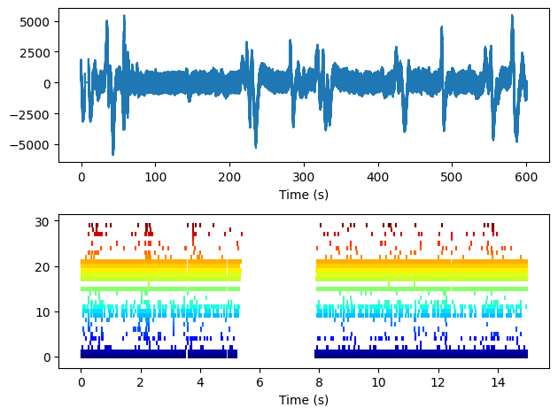
Plexon file

If you have Plexon files, you can use EphysReader in the exact same way:

Show code cell content

Hide code cell content

import urllib
distantfile = "https://web.gin.g-node.org/NeuralEnsemble/ephy_testing_data/raw/master/plexon/File_plexon_3.plx"
urllib.request.urlretrieve(distantfile, "File_plexon_3.plx")

('File_plexon_3.plx', <http.client.HTTPMessage at 0x7fc14b153bc0>)

data = nap.EphysReader("File_plexon_3.plx", format="PlexonIO");

Show code cell output

Hide code cell output

Parsing data blocks:   0%|          | 0/2523688 [00:00<?, ?it/s]

Parsing data blocks:  94%|█████████▍| 2382192/2523688 [00:00<00:00, 23820636.48it/s]

Parsing data blocks:  98%|█████████▊| 2484268/2523688 [00:00<00:00, 23858456.33it/s]

Finalizing data blocks:   0%|          | 0/3 [00:00<?, ?it/s]

Finalizing data blocks for type 1:   0%|          | 0/31 [00:00<?, ?it/s]

Finalizing data blocks for type 1:  61%|██████▏   | 19/31 [00:00<00:00, 172.26it/s]

Finalizing data blocks for type 1: 100%|██████████| 31/31 [00:00<00:00, 184.41it/s]

Finalizing data blocks:  33%|███▎      | 1/3 [00:00<00:00,  5.87it/s]

Finalizing data blocks for type 4: 0it [00:00, ?it/s]

Finalizing data blocks for type 4: 0it [00:00, ?it/s]

Finalizing data blocks for type 5:   0%|          | 0/1 [00:00<?, ?it/s]

Finalizing data blocks for type 5: 100%|██████████| 1/1 [00:00<00:00, 12.29it/s]

Finalizing data blocks: 100%|██████████| 3/3 [00:00<00:00, 11.68it/s]

Parsing signal channels:   0%|          | 0/1 [00:00<?, ?it/s]

Parsing signal channels: 100%|██████████| 1/1 [00:00<00:00, 4181.76it/s]

Parsing spike channels: 0it [00:00, ?it/s]

Parsing spike channels: 30it [00:00, 42784.47it/s]

Parsing event channels: 0it [00:00, ?it/s]

Parsing event channels: 0it [00:00, ?it/s]

print(data)

File_plexon_3
┍━━━━━━━━━┯━━━━━━━━━━┑
│ Key     │ Type     │
┝━━━━━━━━━┿━━━━━━━━━━┥
│ 0:V     │ TsdFrame │
│ TsGroup │ TsGroup  │
┕━━━━━━━━━┷━━━━━━━━━━┙

lfp = data['0:V']
spikes = data['TsGroup']

fig = plt.figure()
ax1 = fig.add_subplot(2, 1, 1)
ax2 = fig.add_subplot(2, 1, 2)
ax1.plot(lfp.t, lfp.d[:])
ax1.set_xlabel("Time (s)")
colors = plt.cm.jet(np.linspace(0, 1, len(spikes)))
ax2.eventplot([spikes[i].t for i in spikes.keys()], colors=colors)
ax2.set_xlabel("Time (s)")
plt.tight_layout()
plt.show()

Saving as NPZ

Pynapple objects have save methods to save them as npz files.

tsd = nap.Tsd(t=np.arange(10), d=np.arange(10))
tsd.save("my_tsd.npz")

print(nap.load_file("my_tsd.npz"))

Time (s)
----------  --
0            0
1            1
2            2
3            3
4            4
5            5
6            6
7            7
8            8
9            9
dtype: int64, shape: (10,)

To load a NPZ to pynapple, it must contain particular set of keys.

print(np.load("my_tsd.npz"))

NpzFile 'my_tsd.npz' with keys: t, d, start, end, type

When the pynapple object have metadata, they are added to the NPZ file.

tsgroup = nap.TsGroup({
    0:nap.Ts(t=[0,1,2]),
    1:nap.Ts(t=[0,1,2])
    }, metadata={"my_label":["a", "b"]})
tsgroup.save("group")

print(np.load("group.npz", allow_pickle=True))

NpzFile 'group.npz' with keys: type, _metadata, t, index, keys...

By default, they are added within the _metadata key:

print(dict(np.load("group.npz", allow_pickle=True))["_metadata"])

{'my_label': array(['a', 'b'], dtype='<U1')}

Memory map

Numpy memory map

Pynapple can work with numpy.memmap.

Show code cell content

Hide code cell content

data = np.memmap("memmap.dat", dtype='float32', mode='w+', shape = (10, 3))

data[:] = np.random.randn(10, 3).astype('float32')

timestep = np.arange(10)

print(type(data))

<class 'numpy.memmap'>

Instantiating a pynapple TsdFrame will keep the data as a memory map.

eeg = nap.TsdFrame(t=timestep, d=data)

print(eeg)

Time (s)              0          1           2
----------  -----------  ---------  ----------
0            0.00825785   1.7054     0.271619
1            1.33453      0.704189  -1.32878
2            0.0440342   -0.111512  -0.263786
3           -1.33752     -1.49339    0.24254
4           -0.490643    -0.561995   1.09902
5            1.08899      0.186225   0.879427
6            1.82997      1.2098     0.0865411
7           -1.49562     -0.234581  -0.430331
8            0.987943     0.701933  -2.6387
9            0.786668    -0.344757  -0.122538
dtype: float32, shape: (10, 3)

We can check the type of eeg.values.

print(type(eeg.values))

<class 'numpy.memmap'>

Zarr

It is possible to use Higher level library like zarr also not directly.

import zarr
zarr_array = zarr.zeros((10000, 5), chunks=(1000, 5), dtype='i4')
timestep = np.arange(zarr_array.shape[0])

tsdframe = nap.TsdFrame(t=timestep, d=zarr_array)

/home/runner/.local/lib/python3.12/site-packages/pynapple/core/utils.py:198: UserWarning: Converting 'd' to numpy.array. The provided array was of type 'Array'.
  warnings.warn(

As the warning suggest, zarr_array is converted to numpy array.

print(type(tsdframe.d))

<class 'numpy.ndarray'>

To maintain a zarr array, you can change the argument load_array to False.

tsdframe = nap.TsdFrame(t=timestep, d=zarr_array, load_array=False)

print(type(tsdframe.d))

<class 'zarr.core.Array'>

Within pynapple, numpy memory map are recognized as numpy array while zarr array are not.

print(type(data), "Is np.ndarray? ", isinstance(data, np.ndarray))
print(type(zarr_array), "Is np.ndarray? ", isinstance(zarr_array, np.ndarray))

<class 'numpy.memmap'> Is np.ndarray?  True
<class 'zarr.core.Array'> Is np.ndarray?  False

Similar to numpy memory map, you can use pynapple functions directly.

ep = nap.IntervalSet(0, 10)
tsdframe.restrict(ep)

Time (s)      0    1    2    3    4
----------  ---  ---  ---  ---  ---
0             0    0    0    0    0
1             0    0    0    0    0
2             0    0    0    0    0
3             0    0    0    0    0
4             0    0    0    0    0
5             0    0    0    0    0
6             0    0    0    0    0
7             0    0    0    0    0
8             0    0    0    0    0
9             0    0    0    0    0
10            0    0    0    0    0
dtype: int32, shape: (11, 5)

group = nap.TsGroup({0:nap.Ts(t=[10, 20, 30])})

sta = nap.compute_event_triggered_average(tsdframe, group, 1, (-2, 3))

print(type(tsdframe.values))
print("\n")
print(sta)

<class 'zarr.core.Array'>


Time (s)
----------  -----------------
-2          [[0. ... 0.] ...]
-1          [[0. ... 0.] ...]
0           [[0. ... 0.] ...]
1           [[0. ... 0.] ...]
2           [[0. ... 0.] ...]
3           [[0. ... 0.] ...]
dtype: float64, shape: (6, 1, 5)

Navigating a dataset

Show code cell content

Hide code cell content

import zipfile

project_path = "MyProject"


if project_path not in os.listdir("."):
  r = requests.get(f"https://osf.io/a9n6r/download", stream=True)
  block_size = 1024*1024
  with open(project_path+".zip", 'wb') as f:
    for data in tqdm.tqdm(r.iter_content(block_size), unit='MB', unit_scale=True,
      total=math.ceil(int(r.headers.get('content-length', 0))//block_size)):
      f.write(data)

  with zipfile.ZipFile(project_path+".zip", 'r') as zip_ref:
    zip_ref.extractall(".")

  0%|          | 0.00/43.0 [00:00<?, ?MB/s]

  2%|▏         | 1.00/43.0 [00:00<00:07, 5.76MB/s]

 19%|█▊        | 8.00/43.0 [00:00<00:01, 34.5MB/s]

 30%|███       | 13.0/43.0 [00:00<00:00, 31.6MB/s]

 44%|████▍     | 19.0/43.0 [00:00<00:00, 39.5MB/s]

 67%|██████▋   | 29.0/43.0 [00:00<00:00, 52.4MB/s]

 86%|████████▌ | 37.0/43.0 [00:00<00:00, 59.0MB/s]

44.0MB [00:00, 51.3MB/s]                          

We can load a folder containing multiple animals and sessions with the Folders class. The method nap.load_folder provides a shortcut.

project = nap.load_folder(project_path)

print(project)

📂 MyProject
└── 📂 sub-A2929

The pynapple IO offers a convenient way of visualizing and navigating a folder based dataset. To visualize the whole hierarchy of Folders, you can call the view property or the expand function.

project.view

📂 MyProject
└── 📂 sub-A2929
    └── 📂 A2929-200711
        ├── 📂 derivatives
        │   ├── position.npz    |        TsdFrame
        │   ├── sleep_ep.npz    |        IntervalSet
        │   ├── wake_ep.npz     |        IntervalSet
        │   └── spikes.npz      |        TsGroup
        ├── 📂 pynapplenwb
        │   └── A2929-200711    |        NWB file
        ├── x_plus_1.npz    |        Tsd
        └── stimulus-fish.npz       |        IntervalSet

Here it shows all the subjects (in this case only A2929), all the sessions and all of the derivatives folders. It shows as well all the NPZ files that contains a pynapple object and the NWB files.

The object project behaves like a nested dictionary. It is then easy to loop and navigate through a hierarchy of folders when doing analyses. In this case, we are gonna take only the session A2929-200711.

session = project["sub-A2929"]["A2929-200711"]
print(session)

📂 A2929-200711
├── 📂 derivatives
├── 📂 pynapplenwb
├── x_plus_1.npz    |        Tsd
└── stimulus-fish.npz       |        IntervalSet

The Folder view gives the path to any object. It can then be easily loaded.

print(project["sub-A2929"]["A2929-200711"]["pynapplenwb"]["A2929-200711"])

A2929-200711
┍━━━━━━━━━━━━━━━━━━━━━━━┯━━━━━━━━━━━━━┑
│ Keys                  │ Type        │
┝━━━━━━━━━━━━━━━━━━━━━━━┿━━━━━━━━━━━━━┥
│ units                 │ TsGroup     │
│ position_time_support │ IntervalSet │
│ epochs                │ IntervalSet │
│ z                     │ Tsd         │
│ y                     │ Tsd         │
│ x                     │ Tsd         │
│ rz                    │ Tsd         │
│ ry                    │ Tsd         │
│ rx                    │ Tsd         │
┕━━━━━━━━━━━━━━━━━━━━━━━┷━━━━━━━━━━━━━┙

JSON sidecar file

A good practice for sharing datasets is to write as many metainformation as possible. Following BIDS specifications, any data files should be accompagned by a JSON sidecar file.

This is possible using the Folder class of pynapple with the argument description.

epoch = nap.IntervalSet(start=np.array([0, 3]), end=np.array([1, 6]))
session.save("stimulus-fish", epoch, description="Fish pictures to V1")

It is then possible to read the description with the doc method of the Folder object.

session.doc("stimulus-fish")

╭─ MyProject/sub-A2929/A2929-200711/stimulus-fish.npz ─╮
│ time : 2026-04-02 18:36:02.971078                    │
│ info : Fish pictures to V1                           │
╰──────────────────────────────────────────────────────╯