Correlograms & ISI

Show code cell content

Hide code cell content

import pynapple as nap
import numpy as np
import matplotlib.pyplot as plt
import seaborn as sns
custom_params = {"axes.spines.right": False, "axes.spines.top": False}
sns.set_theme(style="ticks", palette="colorblind", font_scale=1.5, rc=custom_params)

Let’s generate some data. Here we have two neurons recorded together. We can group them in a TsGroup.

ts1 = nap.Ts(t=np.sort(np.random.uniform(0, 1000, 2000)), time_units="s")
ts2 = nap.Ts(t=np.sort(np.random.uniform(0, 1000, 1000)), time_units="s")
epoch = nap.IntervalSet(start=0, end=1000, time_units="s")
ts_group = nap.TsGroup({0: ts1, 1: ts2}, time_support=epoch)
print(ts_group)

  Index    rate
-------  ------
      0       2
      1       1

Autocorrelograms

We can compute their autocorrelograms meaning the number of spikes of a neuron observed in a time windows centered around its own spikes. For this we can use the function compute_autocorrelogram. We need to specifiy the binsize and windowsize to bin the spike train.

autocorrs = nap.compute_autocorrelogram(
    group=ts_group, binsize=100, windowsize=1000, time_units="ms", ep=epoch  # ms
)
print(autocorrs)

           0     1
-0.9  1.0200  0.91
-0.8  0.9675  0.94
-0.7  0.9275  1.02
-0.6  0.9600  0.98
-0.5  0.9950  1.00
-0.4  1.0350  0.97
-0.3  1.0500  1.07
-0.2  1.0875  0.98
-0.1  1.0225  1.05
 0.0  0.0000  0.00
 0.1  1.0225  1.05
 0.2  1.0875  0.98
 0.3  1.0500  1.07
 0.4  1.0350  0.97
 0.5  0.9950  1.00
 0.6  0.9600  0.98
 0.7  0.9275  1.02
 0.8  0.9675  0.94
 0.9  1.0200  0.91

The variable autocorrs is a pandas DataFrame with the center of the bins for the index and each column is an autocorrelogram of one unit in the TsGroup.

Cross-correlograms

Cross-correlograms are computed between pairs of neurons.

crosscorrs = nap.compute_crosscorrelogram(
    group=ts_group, binsize=100, windowsize=1000, time_units="ms"  # ms
)
print(crosscorrs)

          0
          1
-0.9  0.900
-0.8  0.905
-0.7  1.025
-0.6  1.030
-0.5  0.975
-0.4  1.005
-0.3  0.940
-0.2  1.015
-0.1  1.025
 0.0  1.110
 0.1  0.975
 0.2  0.945
 0.3  0.980
 0.4  1.060
 0.5  0.940
 0.6  1.015
 0.7  0.940
 0.8  1.005
 0.9  1.095

Column name (0, 1) is read as cross-correlogram of neuron 0 and 1 with neuron 0 being the reference time.

Event-correlograms

Event-correlograms count the number of event in the TsGroup based on an event timestamps object.

eventcorrs = nap.compute_eventcorrelogram(
    group=ts_group, event = nap.Ts(t=[0, 10, 20]), binsize=0.1, windowsize=1
    )
print(eventcorrs)

             0         1
-0.9  0.000000  4.444444
-0.8  0.000000  0.000000
-0.7  0.000000  0.000000
-0.6  0.000000  0.000000
-0.5  0.000000  0.000000
-0.4  0.000000  0.000000
-0.3  0.000000  0.000000
-0.2  0.000000  0.000000
-0.1  0.000000  0.000000
 0.0  0.000000  0.000000
 0.1  0.000000  0.000000
 0.2  2.222222  0.000000
 0.3  0.000000  0.000000
 0.4  0.000000  0.000000
 0.5  0.000000  8.888889
 0.6  0.000000  0.000000
 0.7  0.000000  0.000000
 0.8  0.000000  4.444444
 0.9  0.000000  0.000000

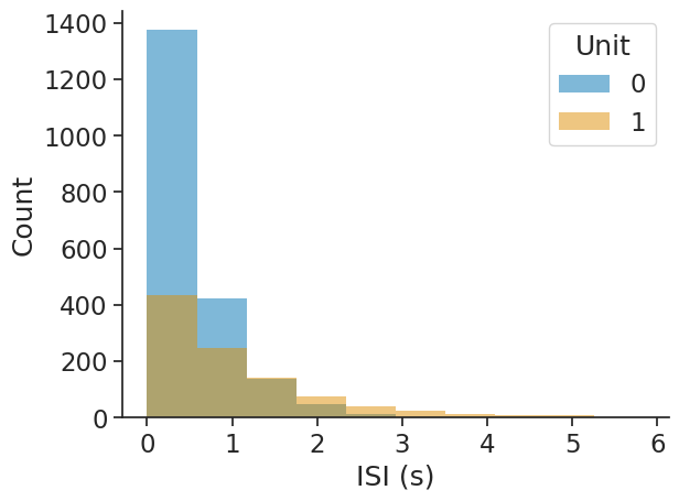
Interspike interval (ISI) distribution

The interspike interval distribution shows how the time differences between subsequent spikes (events) are distributed. The input can be any object with timestamps. Passing epochs restricts the computation to the given epochs. The output will be a dataframe with the bin centres as index and containing the corresponding ISI counts per unit.

isi_distribution = nap.compute_isi_distribution(
    data=ts_group, bins=10, epochs=epoch
    )
print(isi_distribution)

             0    1
0.275651  1344  428
0.826779   432  238
1.377907   153  133
1.929035    40   82
2.480163    19   51
3.031292     7   28
3.582420     2   19
4.133548     1   11
4.684676     1    7
5.235804     0    2

Show code cell source

Hide code cell source

for col in isi_distribution.columns:
    plt.bar(
        isi_distribution.index,
        isi_distribution[col].values,
        width=np.diff(isi_distribution.index).mean(),
        alpha=0.5,
        label=col,
        align='center',
        edgecolor='none'
    )
plt.xlabel("ISI (s)")
plt.ylabel("Count")
plt.legend(title="Unit")
plt.show()

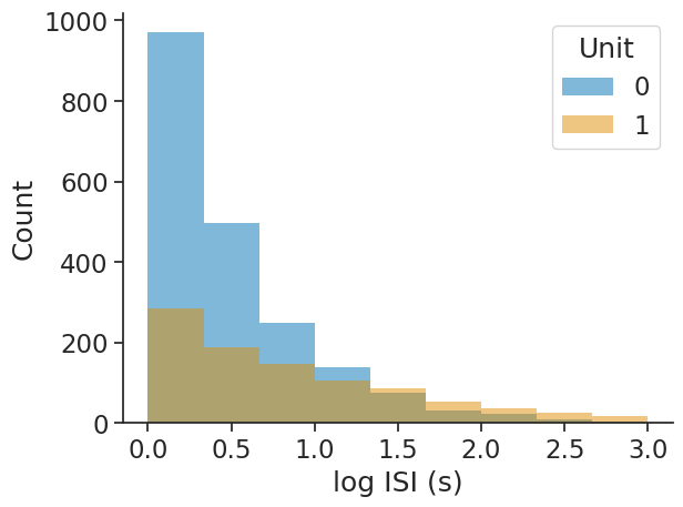
The bins argument allows for choosing either the number of bins as an integer or the bin edges as an array directly:

isi_distribution = nap.compute_isi_distribution(
    data=ts_group, bins=np.linspace(0, 3, 10), epochs=epoch
    )
print(isi_distribution)

             0    1
0.166667  1014  287
0.500000   448  198
0.833333   258  141
1.166667   134  104
1.500000    79   69
1.833333    30   56
2.166667    10   49
2.500000    14   17
2.833333     5   28

Show code cell source

Hide code cell source

for col in isi_distribution.columns:
    plt.bar(
        isi_distribution.index,
        isi_distribution[col].values,
        width=np.diff(isi_distribution.index).mean(),
        alpha=0.5,
        label=col,
        align='center',
        edgecolor='none'
    )
plt.xlabel("log ISI (s)")
plt.ylabel("Count")
plt.legend(title="Unit")
plt.show()

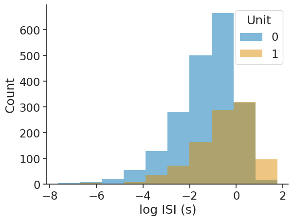
The log_scale argument allows for applying the log-transform to the ISIs:

isi_distribution = nap.compute_isi_distribution(
    data=ts_group, bins=10, log_scale=True, epochs=epoch
    )
print(isi_distribution)

             0    1
-8.799078    1    0
-7.693194    1    2
-6.587311    9    1
-5.481428   15    1
-4.375545   55   13
-3.269662  156   55
-2.163778  437  115
-1.057895  740  267
 0.047988  534  374
 1.153871   51  171

Show code cell source

Hide code cell source

for col in isi_distribution.columns:
    plt.bar(
        isi_distribution.index,
        isi_distribution[col].values,
        width=np.diff(isi_distribution.index).mean(),
        alpha=0.5,
        label=col,
        align='center',
        edgecolor='none'
    )
plt.xlabel("log ISI (s)")
plt.ylabel("Count")
plt.legend(title="Unit")
plt.show()